Links forward

Logistic growth

We have seen many examples of exponential population growth based on an equation

\[ \dfrac{dx}{dt} = kx, \]

saying intuitively that a larger population produces proportionately more offspring.

However, as we have discussed, exponential growth cannot continue forever in a finite ecosystem. There are always limits to growth. One way to model ecological constraints is by adding an extra factor corresponding to the carrying capacity \(R\) of the ecosystem:

\[ \dfrac{dx}{dt} = kx \Bigl( 1 - \dfrac{x}{R} \Bigr). \]

Here \(k\) (the continuous growth rate) and \(R\) are constants. This model is called a logistic model of growth. As \(x\) increases from 0 to \(R\), the factor \(1-\dfrac{x}{R}\) decreases from 1 to 0, expressing the idea that as the population increases towards carrying capacity, growth becomes increasingly difficult; at carrying capacity, growth drops to zero.

Differential equations of this type can be solved explicitly, as we now illustrate.

Suppose there are initially 10 rabbits on an island with a carrying capacity of 1000. In the absence of ecological constraints, the rabbits reproduce with a growth rate of 2. Following the logistic model, we have

\[ \dfrac{dx}{dt} = 2 x \Bigl( 1 - \dfrac{x}{1000} \Bigr) = \dfrac{x (1000 - x)}{500}. \]

Using the fact that \(\dfrac{dx}{dt} \cdot \dfrac{dt}{dx} = 1\) gives

\[ \dfrac{dt}{dx} = \dfrac{500}{x(1000 - x)}. \]

In order to integrate this expression we write it in terms of partial fractions, setting

\[ \dfrac{500}{x(1000 - x)} = \dfrac{A}{x} + \dfrac{B}{1000 - x} \]

and solving for \(A\) and \(B\). Cross-multiplying gives \(500 = A(1000 - x) + Bx\); so we obtain \(A = B = \dfrac{1}{2}\). Thus we can write

\[ \dfrac{dt}{dx} = \dfrac{1}{2x} + \dfrac{1}{2(1000 - x)}. \]

We may antidifferentiate term-by-term to obtain

\begin{align*} t &= \dfrac{1}{2} \log_e x - \dfrac{1}{2} \log_e (1000 - x) + c \\ &= \dfrac{1}{2} \log_e \Bigl(\dfrac{x}{1000-x}\Bigr) + c, \end{align*}

where \(c\) is a constant. Rearranging this equation we obtain

\[ e^{2(t-c)} = \dfrac{x}{1000-x}. \]

Substituting the initial condition \(t=0\), \(x=10\) gives \(e^{-2c} = \dfrac{1}{99}\), so we have

\[ \dfrac{1}{99} e^{2t} = \dfrac{x}{1000 - x}. \]

Solving now for \(x\) gives

\[ x = \dfrac{1000}{99 e^{-2t} + 1}. \]

This is the desired result. As \(t\) increases towards infinity, \(e^{-2t}\) approaches 0, so the denominator approaches 1, and therefore \(x\) approaches the carrying capacity of 1000.

Detailed description

Using the same technique, it can be shown that the general logistic model

\[ \dfrac{dx}{dt} = kx \Bigl( 1 - \dfrac{x}{R} \Bigr), \]

with \(k, R\) constants, has general solution

\[ x = \dfrac{R}{e^{-k(t-c)} + 1}, \]

where \(c\) is a constant.

Functions of this type are often called logistic functions. The simplest such function is

\[ f(t) = \dfrac{1}{e^{-t} + 1}, \]

which has the following graph.

Detailed description

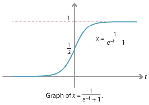
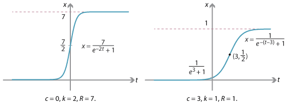
The next two graphs give further examples of logistic functions, with different values of \(k\), \(R\) and \(c\).

Detailed description

Next page - History and applications - World population