Answers to exercises
Exercise 1
- Let \(X\) be the number of winning wrappers in one week (7 days). Then \(X \stackrel{\mathrm{d}}{=} \mathrm{Bi}(7,\frac{1}{6})\).
- \(\Pr(X = 0) = \bigl(\dfrac{5}{6}\bigr)^7 \approx 0.279\).
- The purchases are assumed to be independent, and hence the outcome of the first six days is irrelevant. The probability of a winning wrapper on any given day (including on the seventh day) is \(\dfrac{1}{6}\).
- Let \(Y\) be the number of winning wrappers in six weeks (42 days). Then \(Y \stackrel{\mathrm{d}}{=} \mathrm{Bi}(42,\frac{1}{6})\). Hence, \begin{align*} \Pr(Y \geq 3) &= 1 - \Pr(Y \leq 2) \\ &= 1 - \bigl[\Pr(Y=0) + \Pr(Y=1) + \Pr(Y=2)\bigr] \\ &= 1 - \bigl[\bigl(\tfrac{5}{6}\bigr)^{42} + 42 \times \tfrac{1}{6} \times \bigl(\tfrac{5}{6}\bigr)^{41} + 861 \times \bigl(\tfrac{1}{6}\bigr)^2 \times \bigl(\tfrac{5}{6}\bigr)^{40}\bigr] \\ &\approx 1 - \bigl[0.0005 + 0.0040 + 0.0163\bigr] \approx 0.979. \end{align*} This could also be calculated with the help of the \(\sf \text{BINOM.DIST}\) function in Excel.
- Let \(U\) be the number of winning wrappers in \(n\) purchases. Then \(U \stackrel{\mathrm{d}}{=} \mathrm{Bi}(n,\frac{1}{6})\) and so \begin{align*} \Pr(U \geq 1) \geq 0.95 \ &\iff\ 1 - \Pr(U = 0) \geq 0.95 \\ &\iff\ \Pr(U = 0) \leq 0.05 \\ &\iff\ \bigl(\tfrac{5}{6}\bigr)^n \leq 0.05 \\ &\iff\ n\,\log_e\bigl(\tfrac{5}{6}\bigr) \leq \log_e(0.05) \\ &\iff\ n \geq \dfrac{\log_e(0.05)}{\log_e\bigl(\tfrac{5}{6}\bigr)} \approx 16.431. \end{align*} Hence, he needs to purchase a bar every day for 17 days.
Exercise 2
- Binomial.
- Not binomial. The weather from one day to the next is not independent. Even though, for example, the chance of rain on a day in March may be 0.1 based on long-term records for the city, the days in a particular fortnight are not independent.
- Not binomial. When sampling without replacement from a small population of tickets, the chance of a 'success' (in this case, a blue ticket) changes with each ticket drawn.
- Not binomial. There is likely to be clustering within classes; the students within a class are not independent from each other.
- Binomial.
Exercise 3
This problem is like that of Casey and the winning wrappers. Let \(X\) be the number of sampled quadrats containing the species of interest. We assume that \(X \stackrel{\mathrm{d}}{=} \mathrm{Bi}(n,k)\). We want \(\Pr(X \geq 1) \geq 0.9\), since we only need to observe the species in one quadrat to know that it is present in the forest. We have
\begin{align*} \Pr(X \geq 1) \geq 0.9 \ &\iff\ \Pr(X = 0) \leq 0.1 \\ &\iff\ (1-k)^n \leq 0.1 \\ &\iff\ n \geq \dfrac{\log_e(0.1)}{\log_e(1-k)}. \end{align*}For example: if \(k = 0.1\), we need \(n \geq 22\); if \(k=0.05\), we need \(n \geq 45\); if \(k=0.01\), we need \(n \geq 230\).
Exercise 4
-
\(p\) 0.01 0.05 0.2 0.35 0.5 0.65 0.8 0.95 0.99 \(\mu_X\) 0.2 1 4 7 10 13 16 19 19.8 \(\mathrm{sd}(X)\) 0.445 0.975 1.789 2.133 2.236 2.133 1.789 0.975 0.445
- The standard deviation is smallest when \(|p-0.5|\) is largest; in this set of distributions, when \(p=0.01\) and \(p = 0.99\). The standard deviation is largest when \(p = 0.5\).
Exercise 5
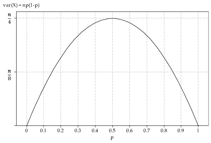
- The graph of the variance of \(X\) as a function of \(p\) is as follows.

Figure 2: Variance of \(X\) as a function of \(p\), where \(X \stackrel{\mathrm{d}}{=} \mathrm{Bi}(n,p)\).
- The variance function is \(f(p) = np(1-p)\). So \(f'(p) = n(1-2p)\). Hence \(f'(p) = 0\) when \(p = 0.5\), and this is clearly a maximum.
- When \(p = 0.5\), we have \(\mathrm{var}(X) = \dfrac{n}{4}\) and \(\mathrm{sd}(X) = \dfrac{\sqrt{n}}{2}\).
Exercise 6
Yes, it is true that, as \(n\) tends to infinity, the largest value of \(p_X(x)\) tends to zero. We will not prove this explicitly, but make the following two observations.
- First consider the case where \(p = 0.5\) and \(n\) is even; let \(n=2m\). The largest value of \(p_X(x)\) occurs when \(x = \dfrac{n}{2} = m\) (see figure 2, for example). This probability is given by
\[
p_X(m) = \dbinom{2m}{m}\, \dfrac{1}{4^m}.
\]
This tends to zero as \(m\) tends to infinity. Proving this fact is beyond the scope of the curriculum (it can be done using Stirling's formula, for example), but evaluating the probabilities for large values of \(m\) will suggest that it is true:
- for \(m=1000\), \(p_X(m) \approx 0.0178\)
- for \(m=10\ 000\), \(p_X(m) \approx 0.0056\)
- for \(m=100\ 000\), \(p_X(m) \approx 0.0018\)
- for \(m=1\ 000\ 000\), \(p_X(m) \approx 0.0006\).
- In general, for \(X \stackrel{\mathrm{d}}{=} \mathrm{Bi}(n,p)\), we have \(\mathrm{sd}(X) = \sqrt{np(1-p)}\). As \(n\) tends to infinity, the standard deviation grows larger and larger, which means that the distribution is more and more spread out, leading to the largest probability gradually diminishing in size.
