Content
Calculating confidence intervals
An approximate standard Normal distribution
We have seen how the distribution of sample proportions approximates a Normal distribution, for large \(n\). The module Exponential and normal distributions shows how any Normal distribution can be standardised, in the following way, to give a standard Normal distribution:
If \(Y \stackrel{\mathrm{d}}{=} \mathrm{N}(\mu,\sigma^2)\) and \(Z = \dfrac{Y-\mu}{\sigma}\), then \(Z \stackrel{\mathrm{d}}{=} \mathrm{N}(0,1)\).
The standard Normal distribution has mean 0 and variance 1. A random variable with this distribution is usually denoted by \(Z\). That is, \(Z \stackrel{\mathrm{d}}{=} \mathrm{N}(0,1)\).
Consider then a standardisation of \(\hat{P}\). We know that \(\mathrm{E}(\hat{P}) = p\) and \(\mathrm{sd}(\hat{P}) = \sqrt{\dfrac{p(1-p)}{n}}\), and we know that \(\hat{P}\) is approximately Normally distributed if \(n\) is large. What is the distribution of the random variable
\[ \dfrac{\hat{P}-p}{\sqrt{\dfrac{1}{n}p(1-p)}}, \]obtained by standardising \(\hat{P}\)?
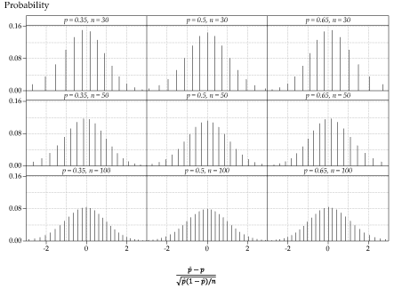
This is illustrated in stages by figures 15, 16 and 17. The distributions in the same position represent the same values of \(p\) and \(n\), as shown by the labelling of the panels.
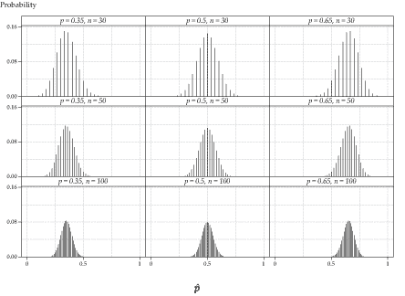
Figure 15: Distribution of \(\hat{P}\), for various values of \(p\) and \(n\).
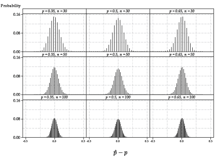
Figure 16: Distribution of \(\hat{P}-p\), for various values of \(p\) and \(n\).

Detailed description
Figure 17: Distribution of the standardisation of \(\hat{P}\), for various values of \(p\) and \(n\).
figure 15 shows the distribution of the sample proportion \(\hat{P}\) in nine different cases, one for each combination of \(p = 0.35, 0.5, 0.65\) and \(n = 30, 50, 100\).
figure 16 shows the distribution of \(\hat{P}-p\) in each of the nine cases. Using the general fact that \(\mathrm{E}(aX+b) = a\,\mathrm{E}(X) + b\), we have \(\mathrm{E}(\hat{P}-p) = p - p = 0\). Further, the general result \(\mathrm{var}(aX+b) = a^2\,\mathrm{var}(X)\) tells us that transforming a random variable by adding a constant leaves the variance unchanged. Hence, \(\mathrm{var}(\hat{P}-p) = \mathrm{var}(\hat{P})\) and so \(\mathrm{sd}(\hat{P}-p) = \mathrm{sd}(\hat{P})\).
So by subtracting the mean \(p\) from \(\hat{P}\), we find that all the distributions are centred at 0, but the spread of each distribution is the same as that of the corresponding distribution in figure 15.
figure 17 shows the distributions obtained when we complete the standardisation, by dividing the random variable \(\hat{P}-p\) by its standard deviation. We are now looking at the distribution of
\[ \dfrac{\hat{P}-p}{\sqrt{\dfrac{1}{n}p(1-p)}}. \]Now all the distributions have the same centre and spread. More specifically,
\begin{align*} \mathrm{E}\Biggl(\dfrac{\hat{P}-p}{\sqrt{\dfrac{1}{n}p(1-p)}}\Biggr) &= 0 \\ \mathrm{sd}\Biggl(\dfrac{\hat{P}-p}{\sqrt{\dfrac{1}{n}p(1-p)}}\Biggr) &= 1. \end{align*}Exercise 4
Confirm that
- \(\mathrm{E}\Biggl(\dfrac{\hat{P}-p}{\sqrt{\dfrac{1}{n}p(1-p)}}\Biggr) = 0\)
- \(\mathrm{sd}\Biggl(\dfrac{\hat{P}-p}{\sqrt{\dfrac{1}{n}p(1-p)}}\Biggr) = 1\).
We know the mean and standard deviation of the standardised random variable, and it is approximately Normally distributed. Putting all this together we can say that, for large \(n\),
\[ \dfrac{\hat{P}-p}{\sqrt{\dfrac{1}{n}p(1-p)}} \stackrel{\mathrm{d}}{\approx} \mathrm{N}(0,1). \]That is, for large \(n\), the distribution of the standardised random variable is approximately the standard Normal distribution.
This standardisation proves crucial in obtaining a confidence interval for the unknown \(p\), when we have an observation from the binomial distribution \(\mathrm{Bi}(n,p)\), as we now show.
Calculating a 95% confidence interval with the Normal approximation
The crucial point to see in figure 17 is that all of the distributions are approximately the same, regardless of the values of \(p\) and \(n\). This is especially important, since we don't know the value of \(p\); we are trying to estimate it.
As discussed in the module Exponential and normal distributions, for a Normal random variable \(X \stackrel{\mathrm{d}}{=} \mathrm{N}(\mu,\sigma^2)\), about 95% of the distribution is within two standard deviations of the mean. That is,
\[ \Pr(\mu-2\sigma < X < \mu+2\sigma) \approx 0.95. \]Hence, for a random variable with the standard Normal distribution, \(Z \stackrel{\mathrm{d}}{=} \mathrm{N}(0,1)\), we have \(\Pr(-2 < Z < 2) \approx 0.95\). To be more precise:
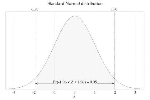
\[ \Pr(-1.96 < Z < 1.96) = 0.95. \]This is illustrated in figure 18.
Detailed description
Figure 18: The standard Normal distribution, \(Z \stackrel{\mathrm{d}}{=} \mathrm{N}(0,1)\).
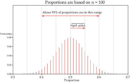
figure 19 shows the distribution of the sample proportion \(\hat{P}\) for sample size \(n=100\) and population proportion \(p=0.5\) (or, equivalently, for observations from the \(\mathrm{Bi}(100,0.5)\) distribution). The standard deviation of \(\hat{P}\) is shown in the figure. Only a small percentage of the sample proportions are more than two standard deviations away from \(p = 0.5\). About 95% of the sample proportions are within two standard deviations of \(p\).
Detailed description
Figure 19: Distribution of the sample proportion based on \(n=100\) and \(p=0.5\).
Similarly, for each of the distributions of standardised sample proportions in figure 17, about 95% of the distribution is within two standard deviations of the mean. Since each of the standardised sample proportions has a distribution that can be approximated by the standard Normal distribution, we can state that, for large \(n\),
\[ \Pr\Biggl(-1.96 < \dfrac{\hat{P}-p}{\sqrt{\dfrac{1}{n}p(1-p)}} < 1.96\Biggr) \approx 0.95. \]We multiply through by \(\sqrt{\dfrac{p(1-p)}{n}}\) to obtain
\[ \Pr\Biggl(-1.96\sqrt{\dfrac{p(1-p)}{n}} < \hat{P}-p < 1.96\sqrt{\dfrac{p(1-p)}{n}}\Biggr) \approx 0.95. \]In other words, the distance between \(\hat{P}\) and \(p\) will be no more than \(1.96 \sqrt{\dfrac{p(1-p)}{n}}\) for 95% of sample proportions.
One further rearrangement gives
\[ \Pr\Biggl(\hat{P}-1.96\sqrt{\dfrac{p(1-p)}{n}} < p < \hat{P}+1.96\sqrt{\dfrac{p(1-p)}{n}}\Biggr) \approx 0.95. \]It is really important to reflect on this probability statement. Note that it has \(p\) in the centre of the inequalities. The population parameter \(p\) does not vary: it is fixed, but unknown. The random element in this probability statement is the random interval around \(p\).
This forms the basis for the approximate 95% confidence interval for the true proportion \(p\). In a given case, we have just a single observation from the \(\mathrm{Bi}(n,p)\) distribution. We then find the observed value \(\hat{p}\) of \(\hat{P}\), and obtain the observed value of the random interval, which we call the 95% confidence interval.
This gives us a 95% confidence interval for \(p\):
\[ \Biggl(\hat{p}-1.96\sqrt{\dfrac{p(1-p)}{n}},\ \hat{p}+1.96\sqrt{\dfrac{p(1-p)}{n}}\Biggr). \]However, a problem remains. The unknown parameter is still present in the formula! This seems unfortunate, to say the least; the very parameter we are seeking to estimate is present in a formula that reflects the precision of our estimate.
The solution is to make a further approximation and substitute \(\hat{p}\) for \(p\) in the expression for the standard deviation of \(\hat{P}\).
Hence, an approximate 95% confidence interval for \(p\) is given by
\[ \Biggl(\hat{p}-1.96\sqrt{\dfrac{\hat{p}(1-\hat{p})}{n}},\ \hat{p}+1.96\sqrt{\dfrac{\hat{p}(1-\hat{p})}{n}}\Biggr) \qquad\qquad\qquad(\ast) \]or, equivalently,
\[ \hat{p} \pm 1.96\sqrt{\dfrac{\hat{p}(1-\hat{p})}{n}}. \]It is reasonable at this point to ask: How do we know that the Normal approximation is adequate when we have substituted \(\hat{p}\) for \(p\), as described? We provide an informal answer to this sensible question in figure 20, by showing the distributions of
\[ \dfrac{\hat{P}-p}{\sqrt{\dfrac{1}{n}\hat{P}(1-\hat{P})}} \]for the same values of \(p\) and \(n\) as in figure 17. Reassuringly, the two figures 17 and 20 are almost indistinguishable. It is true that, for large \(n\),
\[ \dfrac{\hat{P}-p}{\sqrt{\dfrac{1}{n}\hat{P}(1-\hat{P})}} \stackrel{\mathrm{d}}{\approx} \mathrm{N}(0,1). \]This confirms that, for large \(n\), the confidence interval (\(\ast\)) derived above is a reasonable approximation.
Detailed description
Figure 20: Distribution of \(\dfrac{\hat{P}-p}{\sqrt{\dfrac{1}{n}\hat{P}(1-\hat{P})}}\), for various values of \(p\) and \(n\); compare with figure 17.
Keep in mind that the value of 1.96 in the calculation of the confidence interval comes from the use of the standard Normal distribution, and corresponds to a central area of 95%. This is the appropriate factor because the chosen level of confidence is 95%.
We have used the phrase 'for large \(n\)' frequently, and relied on visual impressions from various distributions to get a sense of what may be adequately large for the approximation to be satisfactory in practice. In fact, the adequacy depends on both \(n\) and \(p\). A guideline often given is that:
If \(X \stackrel{\mathrm{d}}{=} \mathrm{Bi}(n,p)\) and the observation we are using for the approximate confidence interval is \(x\), then we require both \(x\) and \(n-x\) to be greater than 10.
Example: Mobile-phone use among children
A recent large survey of a random sample of Australian children asked about mobile-phone ownership in three age groups. The following table shows the number of mobile-phone owners and the total number of children surveyed for each age group.
| Age group (years) | Number of mobile owners | Number surveyed |
|---|---|---|
| 5–8 | 50 | 2150 |
| 9–11 | 544 | 2530 |
| 12–14 | 918 | 1250 |
Calculate an approximate 95% confidence interval for the true proportion of mobile-phone owners in each group.
Solution
These data easily meet the guideline for the Normal approximation to be adequate.
In the 5–8 age group, we have \(\hat{p} = \dfrac{50}{2150} = 0.0233\) and so
\[ 1.96\sqrt{\dfrac{\hat{p}(1-\hat{p})}{n}} = 1.96\sqrt{\dfrac{0.0233(1-0.0233)}{2150}} = 0.00637. \]Hence, the 95% confidence interval is \(0.0233 \pm 0.00637\), or \((0.0169, 0.0296)\). In percentage terms, the confidence interval is \(1.69\%\) to \(2.96\%\).
It is important to learn the real meaning of this confidence interval. As discussed in the section Confidence intervals, we cannot really say that the chance that the unknown percentage is between \(1.69\%\) and \(2.96\%\) is equal to 0.95. Once we have the data and the actual calculated interval, there is no randomness involved: the unknown percentage is a fixed number, not a random variable. Rather, we can say that we have calculated an interval using a process that, in a long run of repeated instances of the study under the same circumstances, would produce intervals that contained the unknown percentage in 95% of cases, on average.
For the 9–11 age group, we have \(\hat{p} = \dfrac{544}{2530} = 0.215\) and so
\[ 1.96\sqrt{\dfrac{\hat{p}(1-\hat{p})}{n}} = 1.96\sqrt{\dfrac{0.215(1-0.215)}{2530}} = 0.0160. \]Hence, the 95% confidence interval is \(0.215 \pm 0.0160\), or \((0.199, 0.231)\). In percentage terms, the confidence interval is \(19.9\%\) to \(23.1\%\).
For the 12–14 age group, we have \(\hat{p} = \dfrac{918}{1250} = 0.734\) and so
\[ 1.96\sqrt{\dfrac{\hat{p}(1-\hat{p})}{n}} = 1.96\sqrt{\dfrac{0.734(1-0.734)}{1250}} = 0.0245. \]Hence, the 95% confidence interval is \(0.734 \pm 0.0245\), or \((0.710, 0.759)\). In percentage terms, the confidence interval is \(71.0\%\) to \(75.9\%\).
Exercise 5
Casey buys a Venus chocolate bar every day for 180 days, during a promotion promising that 'one is six wrappers is a winner'. From these 180 purchases, Casey gets 20 winning wrappers.
- What is the proportion of winning wrappers Casey expects to get, if the advertised claim is true? How many winning wrappers would this imply, for Casey?
- What is the proportion of winning wrappers in Casey's sample?
- Find an approximate 95% confidence interval for the true proportion of winning wrappers, based on Casey's sample of Venus bars.
- Casey feels he has missed out, and suspects that the true proportion of winners is not one in six. Comment on this, based on Casey's sample of Venus bars.
- What assumptions have been made about Casey's sample of Venus bar wrappers?
Next page - Content - More on calculating confidence intervals
