Content

Linear transformations and matrices

We will now take a more algebraic approach to transformations of the plane.

As it turns out, matrices are very useful for describing transformations. Whenever we have a $2 \times 2$ matrix of real numbers

\[ M = \begin{bmatrix} a & b \\ c & d \end{bmatrix}, \]

we can naturally define a plane transformation $T_M : \mathbb{R}^2 \rightarrow \mathbb{R}^2$ by

\[ T_M ({\bf v}) = M {\bf v}. \]

That is, $T_M$ takes a vector ${\bf v}$ and multiplies it on the left by the matrix $M$. If ${\bf v}$ is the position vector of the point $(x,y)$, then

\[ T_M ({\bf v}) = T_M \left( \begin{bmatrix} x \\ y \end{bmatrix} \right) = M \begin{bmatrix} x \\ y \end{bmatrix} = \begin{bmatrix} a & b \\ c & d \end{bmatrix} \begin{bmatrix} x \\ y \end{bmatrix} = \begin{bmatrix} ax+by \\ cx+dy \end{bmatrix} \]

or equivalently, $T_M (x,y) = (ax+by, cx+dy)$.

(Note that here we used the notation $(x,y)$ and $\begin{bmatrix} x \\ y \end{bmatrix}$ interchangeably; we will be doing this throughout this module.)

As it turns out, matrices give us a powerful systematic way to describe a wide variety of transformations: they can describe rotations, reflections, dilations, and much more.

Note that $T_M(1,0)$ and $T_M(0,1)$ are precisely the columns of the matrix $M$. This is an important fact, which we will discuss later.

While every matrix describes a plane transformation, not every plane transformation can be described by a matrix. Matrices correspond to a specific type of plane transformation which sends $(x,y)$ to $(ax+by,cx+dy)$, for some real numbers $a,b,c,d$.

A transformation $T_M$ arising from a matrix $M$ obeys some "distributive laws". For any $2 \times 2$ matrix $M$ and vectors ${\bf v}$ and ${\bf w}$ in $\mathbb{R}^2$, it is true that

\[ M \left( {\bf v} + {\bf w} \right) = M {\bf v} + M {\bf w} \quad \text{and hence} \quad T_M \left( {\bf v} + {\bf w} \right) = T_M ({\bf v}) + T_M ({\bf w}). \]

Moreover, for any real number (scalar) $c$,

\[ M \left( c {\bf v} \right) = c M {\bf v} \quad \text{and hence} \quad T_M \left( c {\bf v} \right) = c T_M ( {\bf v} ). \]

In fact, if a function $F: \mathbb{R}^2 \rightarrow \mathbb{R}^2$ satisfies these two distributive laws, then it must arise from a matrix. Why? If $F({\bf v} + {\bf w}) = F({\bf v}) + F({\bf w})$ and $F(c{\bf v}) = cF({\bf v})$, then for any point $(x,y)$,

\begin{align*} F \begin{bmatrix} x \\ y \end{bmatrix} &= F \left( \begin{bmatrix} x \\ 0 \end{bmatrix} + \begin{bmatrix} 0 \\ y \end{bmatrix} \right) = F \begin{bmatrix} x \\ 0 \end{bmatrix} + F \begin{bmatrix} 0 \\ y \end{bmatrix} \quad \text{(using $F({\bf v} + {\bf w}) = F({\bf v}) + F({\bf w})$)} \\ &= x F \begin{bmatrix} 1 \\ 0 \end{bmatrix} + y F \begin{bmatrix} 0 \\ 1 \end{bmatrix} \quad \text{(using $F(c{\bf v}) = cF({\bf v})$)} \end{align*}

Letting $F(1,0) = (a,c)$ and $F(0,1) = (b,d)$ then, we have

\[ F \begin{bmatrix} x \\ y \end{bmatrix} = x \begin{bmatrix} a \\ c \end{bmatrix} + y \begin{bmatrix} b \\ d \end{bmatrix} = \begin{bmatrix} ax+by \\ cx+dy \end{bmatrix} = \begin{bmatrix} a & b \\ c & d \end{bmatrix} \begin{bmatrix} x \\ y \end{bmatrix}, \]

so $F$ corresponds to a matrix.

Therefore, we have two equivalent ways to define linear transformations.

Definition

A plane transformation $F$ is linear if either of the following equivalent conditions holds:

• $F(x,y) = (ax+by,cx+dy)$ for some real $a,b,c,d$. That is, $F$ arises from a matrix.
• For any scalar $c$ and vectors ${\bf v}, {\bf w}$, $F(c{\bf v}) = c F({\bf v})$ and $F({\bf v} + {\bf w}) = F({\bf v}) + F({\bf w})$.

The effect of a linear transformation

Suppose you are given a matrix $M$. You now know that $M$ determines a linear transformation $T_M$. But what does $T_M$ do, geometrically? We will now see a method to analyse this question.

Let's begin by restricting our attention to two vectors: $(1,0)$ and $(0,1)$. These two vectors are sometimes called the standard basis for $\mathbb{R}^2$.

Multiplying any matrix $M = \begin{bmatrix} a & b\\ c & d \end{bmatrix}$ by the standard basis vectors gives its columns: \[ M \begin{bmatrix} 1 \\ 0 \end{bmatrix} = \begin{bmatrix} a & b \\ c & d \end{bmatrix} \begin{bmatrix} 1 \\ 0 \end{bmatrix} = \begin{bmatrix} a \\ c \end{bmatrix} \quad \text{and} \quad M \begin{bmatrix} 0 \\ 1 \end{bmatrix} = \begin{bmatrix} a & b \\ c & d \end{bmatrix} \begin{bmatrix} 0 \\ 1 \end{bmatrix} = \begin{bmatrix} b \\ d \end{bmatrix}. \]

So, just by looking at a matrix $M$, reading down its columns, you can see where $T_M$ sends $(1,0)$ and $(0,1)$. Once you know where $T_M$ sends $(1,0)$ and $(0,1)$, you can use the "distributive" property of linear transformations to see where any other point goes.

For instance, if you want to know where $T_M$ sends $(2,3)$, you could note that $(2,3) = 2 (1,0) + 3 (0,1)$, so that

\[ T_M(2,3) = 2 T_M (1,0) + 3 T_M (0,1). \]

Hence $T_M (2,3)$ is given by $2$ times the first column of $M$, plus $3$ times the second column.

In the $xy$-plane we can consider the unit square, with vertices $(0,0), (1,0), (0,1), (1,1)$. Unit squares tiles the plane, giving a tessellation whose vertices are precisely the points with integer coordinates. Where does $T_M$ send these points?

• $T_M$ sends the origin to the origin (exercise 2).
• $T_M$ sends $(1,0)$ and $(0,1)$ to the vectors given by the first and second columns of $M$.
• $T_M$ sends $(1,1) = (1,0) + (0,1)$, to $T_M(1,0) + T_M(0,1)$, the sum of the two columns of $M$.
• In general, $T_M$ sends $(a,b)$ to $a T_M(1,0) + b T_M (0,1)$.

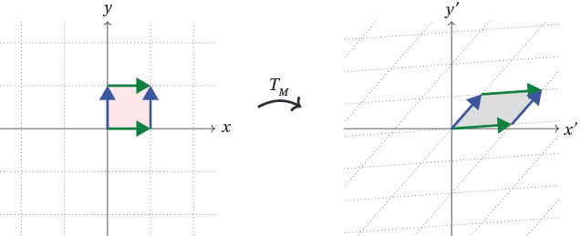
So the unit square is sent by $T_M$ to a parallelogram. The distributive property implies that the whole tessellation of the plane by unit squares is sent by $T_M$ to a tessellation of the plane by parallelograms. We can then draw a picture of the entire transformation $T_M$.

Let us now use these ideas to describe some specific linear transformations.

In the above figure, we draw a parallelogram (shaded grey) with two vectors ${\bf v} = T_M(1,0)$ (green) and ${\bf w} = T_M(0,1)$ (blue) tail-to-tail at the origin. We call this the parallelogram spanned by ${\bf v}$ and ${\bf w}$.

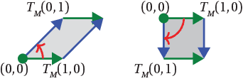
Note that in the two examples above, the parallelograms spanned by $T_M(1,0)$ and $T_M(0,1)$ have different orientations. In the first example, if we consider sweeping around the origin, through the parallelogram, from $T_M(1,0)$ to $T_M(0,1)$, we go anticlockwise; in the second example, we go clockwise. Accordingly, we say the first parallelogram is positively oriented, and the second is negatively oriented.

In the standard unit square, sweeping around the origin from $(1,0)$ to $(0,1)$ goes anticlockwise, so it is positively oriented. So the first example preserved this orientation, and the second example reversed it. In general, we say a linear transformation preserves or reverses orientation accordingly as the parallelogram spanned by $T_M (1,0)$ and $T_M(0,1)$ is positively or negatively oriented.

Composing linear transformations and matrix multiplication

Let's now suppose we have two matrices $M,N$ representing two linear transformations $T_M, T_N$. What happens if we apply one transformation then the other? What is the composition $T_M \circ T_N$?

Let $M = \begin{bmatrix} a & b \\ c & d \end{bmatrix}$ and $N = \begin{bmatrix} e & f \\ g & h \end{bmatrix}$. So

\[ T_M (x,y) = (ax+by, cx+dy) \quad \text{and} \quad T_N (x,y) = (ex+fy, gx+hy). \]

Composing these two functions gives

\begin{align*} T_M \circ T_N (x,y) &= T_M ( T_N (x,y) ) = T_M ( ex+fy, gx+hy ) \\ &= \left( a (ex+fy) + b (gx+hy), \; c (ex+fy) + d (gx+hy) \right) \\ &= \left( (ae+bg) x + (af+bh) y, \; (ce+dg) x + (cf+dh) y \right). \end{align*}

Remembering that $a,b,c,d,e,f,g,h$ are just real constants, this is another linear transformation, and the corresponding matrix is

\[ \begin{bmatrix} ae+bg & af+bh \\ ce+dg & cf+dh \end{bmatrix}. \]

This matrix is precisely the product of the two matrices $M$ and $N$:

\[ MN = \begin{bmatrix} a & b \\ c & d \end{bmatrix} \begin{bmatrix} e & f \\ g & h \end{bmatrix} = \begin{bmatrix} ae+bg & af+bh \\ ce+dg & cf+dh \end{bmatrix}. \]

We conclude that the composition of the linear transformations of $M$ and $N$ is the linear transformation of $MN$, proving the following theorem.

Theorem

For any matrices $M$ and $N$, $T_M \circ T_N = T_{MN}$.

\(\Box\)

This theorem gives us a very quick way to compose linear transformations: just multiply the corresponding matrices!

The identity transformation and identity matrix

Recall the identity transformation $I: \mathbb{R}^2 \rightarrow \mathbb{R}^2$ sends every point to itself, $I(x,y) = (x,y)$. We can now note $I$ is a linear transformation, corresponding to the identity matrix

\[ \text{Id} = \begin{bmatrix} 1 & 0 \\ 0 & 1 \end{bmatrix}. \quad \text{In other words,} \quad T_{\text{Id}} = I. \]

The inverse of a linear transformation and inverse matrices

Recall that a function has an inverse if and only if it is bijective, i.e. injective and surjective. (A function $f: X \rightarrow Y$ is injective if $x \neq y$ implies $f(x) \neq f(y)$; and $f$ is surjective if its image is all of $Y$, i.e. for all $y \in Y$ there exists $x \in X$ such that $f(x) = y$.)

Some transformations of the plane are bijective, and some are not; so some have inverses, and others do not. As we proceed, we will see many examples of transformations that have inverses, and many that don't.

A bijective transformation $F: \mathbb{R}^2 \rightarrow \mathbb{R}^2$, has an inverse $F^{-1} : \mathbb{R}^2 \rightarrow \mathbb{R}^2$. These functions $F$ and $F^{-1}$ "undo" each other. So if $F({\bf x}) = {\bf y}$ then $F^{-1}({\bf y}) = {\bf x}$, and vice versa.

Recall that matrices can have inverses too. If

\[ M = \begin{bmatrix} a & b \\ c & d\end{bmatrix} \quad \text{then} \quad M^{-1} = \frac{1}{ad-bc} \begin{bmatrix} d & -b \\ -c & a \end{bmatrix} \quad \text{(provided $ad-bc \neq 0$).} \]

We say $M^{-1}$ is the inverse of $M$ because $M$ and $M^{-1}$ multiply to give the identity.

If we compose the linear transformations $T_M$ and $T_{M^{-1}}$, we obtain the identity:

\[ T_M \circ T_{M^{-1}} = T_{MM^{-1}} = T_{\text{Id}} = I, \quad T_{M^{-1}} \circ T_M = T_{M^{-1} M} = T_{\text{Id}} = I. \]

Hence $T_M$ and $T_{M^{-1}}$ undo each other; they are inverse transformations.

To show that a function does not have an inverse, one can show that it is not injective, or that it is not surjective. In the following example we do both, giving two solutions.

The following example illustrates a useful technique for finding a linear transformation, from its value at two points.

Next page - Content - Describing geometric transformations algebraically