The Improving Mathematics Education in Schools (TIMES) Project

It is assumed that in Years 1-5, students have had many learning experiences that consider simple and everyday events involving chance, and descriptions of them. They have considered which events are, or may be assumed, more or less likely, and, if events are not more or less likely than others, then they have considered that it is reasonable to assume the events to be equally-likely. They have looked at simple everyday events where one cannot happen if the other happens, and, in contrast, they have thought about simple situations where it is reasonable to assume that the chance of occurrence of an event is not changed by the occurrence of another. They recognise impossible and certain events, and that probabilities range from 0 to 1. They have listed outcomes of chance situations for which equally-likely outcomes may be assumed and represent the equal probabilities using fractions.
Statistics and statistical thinking have become increasingly important in a society that relies more and more on information and calls for evidence. Hence the need to develop statistical skills and thinking across all levels of education has grown and is of core importance in a century which will place even greater demands on society for statistical capabilities throughout industry, government and education.
Statistics is the science of variation and uncertainty. Concepts of probability underpin all of statistics, from handling and exploring data to the most complex and sophisticated models of processes that involve randomness. Statistical methods for analysing data are used to evaluate information in situations involving variation and uncertainty, and probability plays a key role in that process. All statistical models of real data and real situations are based on probability models. Probability models are at the heart of statistical inference, in which we use data to draw conclusions about a general situation or population of which the data can be considered randomly representative.
Probability is a measure, like length or area or weight or height, but a measure of the likeliness or chance of possibilities in some situation. Probability is a relative measure; it is a measure of chance relative to the other possibilities of the situation. Therefore, it is very important to be clear about the situation being considered. Comparisons of probabilities − which are equal, which are not, how much bigger or smaller − are therefore also of interest in modelling chance.
Where do the values of probabilities come from? How can we “find” values? We can model them by considerations of the situation, using information, making assumptions and using probability rules. We can estimate them from data. Almost always we use a combination of assumptions, modelling, data and probability rules.
The concepts and tools of probability pervade analysis of data. Even the most basic exploration and informal analysis involves at least some modelling of the data, and models for data are based on probability. Any interpretation of data involves considerations of variation and therefore at least some concepts of probability.
Situations involving uncertainty or randomness include probability in their models, and analysis of models often leads to data investigations to estimate parts of the model, to check the suitability of the model, to adjust or change the model, and to use the model for predictions.
Thus chance and data are inextricably linked and integrated throughout statistics. However, even though considerations of probability pervade all of statistics, understanding the results of some areas of data analysis requires only basic concepts of probability. The objectives of the chance and probability strand of the F-10 curriculum are to provide a practical framework for experiential learning in foundational concepts of probability for life, for exploring and interpreting data, and for underpinning later developments in statistical thinking and methods, including models for probability and data.
In this module, in the context of understanding chance and its effects in everyday life, we build on the preliminary concepts of chance of Years 1-5 to focus more closely on understanding how chance affects what we observe in simple and familiar situations.
Because such understanding involves concepts of the size (and hence relative size) of probabilities, we describe probabilities using a number of forms, namely fractions, decimals and percentages.
We then consider experiments involving known probabilities to observe the effects of probability on observations and compare what are observed with what is expected. This is carried out with both small and large numbers of repetitions to help students gain an understanding of the effects of probabilities in real situations. Each example experiment can be conducted in real or virtual circumstances. The concepts and effects of probability on observations are experienced through examples of situations familiar and accessible to Year 6 students and that build on concepts and experiences introduced in 1-5.
Before we can begin to describe probabilities, we need to clearly identify the situation and describe the outcomes or events so that there is no confusion and anyone reading or hearing our description will be thinking of the events in the same way as us. Sometimes it is very easy to describe possible events and sometimes there is really only one way of describing them, but in many situations this is not so and careful description is therefore important.
Once we have described the situation and its outcomes or events, we can then think about the probabilities of the outcomes or events. This often requires us to think about which outcomes or events could be assumed to be equally-likely. For a (finite) number of equally-likely outcomes of a simple and everyday situation, we can assign the equal probabilities as fractions, being 1/(total number of outcomes). Sometimes it is straightforward to be able to assume equally-likely and sometimes the assumptions may need more careful identification. For simple situations, if events cannot be assumed to be equally-likely, we may still be able to assign values of probabilities through simple assumptions that are essentially based on the equal-likeliness of number or size. In other situations, we are often able to assign probabilities based on information from an external source or investigation, including assignations based on estimating from observations.
Understanding the types and variety of effects of probability on real observations requires a sound sense of the size of the probabilities. This sense can often be heightened by different expressions for probabilities − as fractions, decimals or percentages. Some people have a preference amongst these, but for many people it is useful to be able to move between these. Hence in the examples below, the probabilities are expressed in each of these three forms.
We will consider situations in which the description of the events is straightforward and assignation of values for the probabilities is also straightforward, with the assumptions being readily accessible for Year 6.
Example A: What colour sweet will you get?
Suppose you have a small box of different coloured sweets, such as M&M’s or Smarties. You give one to your friend by shaking one out of the box onto your friend’s hand. The possible events here are the possible colours of the sweet that lands in your friend’s hand. Whatever colours are possible for the sweets, then this is the list of possible events. For example, the list of possible colours might be (red, yellow, green, blue, orange, brown).
In giving a sweet to your friend by shaking one out of your box of sweets onto your friend’s hand, suppose you have put sweets from a larger container into your small box, and you chose to put in 10 red, 10 yellow, 10 brown, and 10 green and shaken the box well. The possible colours of the sweet you shake from the box into your friend’s hand are these 4 colours. If the box is well shaken, then none of these colours is more likely than the other. So the total probability of 1 is divided into 4 equal bits of probability.
There is a chance of  that your friend will get any of the 4 colours. Equivalently, we say that the chance of each of the colours is 0.25, or that we have a 25% chance of getting a particular colour.
Now suppose you chose to put in 8 red, 8 yellow, 8 brown, 8 green and 8 blue and shaken the box well. The possible colours of the sweet you shake from the box into your friend’s hand are these 5 colours. If the box is well shaken, then none of these colours is more likely than the other. So the total probability of 1 is divided into 5 equal bits of probability. Your friend’s favourite colour is green. There is a chance of  that your friend will get a green one. We can also express this as a chance of 0.2 or a 20% chance of getting a green sweet.
Example B: Throwing one die
In throwing one die, there are 6 possible outcomes. These are the values of the uppermost face and hence the outcomes are the numbers 1, 2, 3, 4, 5, 6. Are any of the faces more likely to come up than any others? A fair die is one for which it is assumed that the 6 faces are equally-likely to be uppermost in a toss of the die. If one or more faces are more likely to come up than others, the die is called a “loaded” die.
If we assume a die is fair, we have 6 possible outcomes all with the same chance of occurring. So we need to divide our total probability of 1 into 6 equal bits of probability. Therefore each bit of probability is  .
.
This probability is not quite as straightforward to express as a decimal or a percentage, so people tend to think just in terms of a fraction for this probability.
Example C: Which ticket will be selected?
Raffles are usually run by people buying numbered (and sometimes coloured) tickets with the tickets being in two parts. The buyers keep one part and the other parts are put into a container with someone picking out a ticket at random from the container. The outcomes of the draw are all the tickets that have been sold. If 100 tickets are sold, the chance of your ticket being picked out is  . This is a 0.01 chance or a 1% chance.
If 1000 tickets are sold, the chance of your ticket being picked out is  . This is a very small chance although 10 times greater than if 10,000 tickets are sold!
Suppose 10 students in your class have volunteered to represent your class for some purpose. To choose one, the 10 names are written on pieces of paper, folded, put in a container which is shaken, and then a piece of paper is drawn at random. The outcomes are the 10 names. Each person has a chance of  , or 0.1 or 10% chance of being chosen. Which way of expressing the chance do you like best?
Example D: Which letter is the most common in the English language?
The inventor of Morse code, Samuel Morse (1791-1872), needed to know how often the different letters occurred in words in the English language so that he could give the simplest codes to the most frequently used letters. He needed to know this for the situation of speech or text because he wanted to be able to code messages. He based his decisions on data he collected from sets of printers’ type, that is, the sets of little blocks of letters that printers then assembled to make words which they put together to print pages. So a printer had to have enough of all the different letters to set up pages for printing. The figures he came up with were:
| 12,000 | E | 2,500 | F |
| 9,000 | T | 2,000 | W, Y |
| 8,000 | A, I, N, O, S | 1,700 | G, P |
| 6,400 | H | 1,600 | B |
| 6,200 | R | 1,200 | V |
| 4,400 | D | 800 | K |
| 4,000 | L | 500 | Q |
| 3,400 | U | 400 | J, X |
| 3,000 | C, M | 200 | Z |
Source: http://www.oxforddictionaries.com/page/frequencyalphabet
Using the above gives the following relative frequencies expressed as percentages. Relative frequencies of categories are the fractions or proportions of observations in the data that fall into each category − see Data Investigation and Interpretation, Year 6.
| 11.3% | E | 2.3% | F |
| 8.5% | T | 1.9% | W, Y |
| 7.5% | A, I, N, O, S | 1.6% | G, P |
| 6% | H | 1.5% | B |
| 5.8% | R | 1.1% | V |
| 4.1% | D | 0.75% | K |
| 3.8% | L | 0.45% | Q |
| 3.2% | U | 0.4% | J, X |
| 2.8% | C, M | 0.2% | Z |
These percentages can be used as estimates of the chances of the different letters in messages, books, magazines etc.
This is different to how often letters appear in vocabulary, because in messages, books, magazines and everyday speech, there are many words that are repeated or used much more than other words. So for word games, it is important to know how often letters appear in vocabulary. An analysis of the letters occurring in the words listed in the main entries of the Concise Oxford Dictionary (11th edition revised, 2004) came up with the following table of relative frequencies expressed as percentages: (based on, and adapted from, http://www.oxforddictionaries.com/page/frequencyalphabet )
| E | 11.2% | M | 3% |
| A | 8.5% | H | 3% |
| R | 7.6% | G | 2.5% |
| I | 7.5% | B | 2% |
| O | 7.2% | F | 1.8% |
| T | 7% | Y | 1.8% |
| N | 6.7% | W | 1.3% |
| S | 5.7% | K | 1.1% |
| L | 5.5% | V | 1% |
| C | 4.5% | X | 0.3% |
| U | 3.6% | Z | 0.3% |
| D | 3.4% | J | 0.2% |
| P | 3.2% | Q | 0.2% |
These percentages can be used as estimates of the probabilities of the different letters in English vocabulary.
Exercise: work out the relative frequencies of the letters in a Scrabble set. How do they compare with the relative frequencies in the table above for English vocabulary?
Effects of probabilities on observations
If we shake out one sweet from a box with a 25% chance of getting any one of 4 colours, we get just one colour. If we put it back and shake out another sweet, we again get just one colour. In Year 4, we considered situations in which it is reasonable to assume that the chance of one occurrence will not be affected by other occurrences. If we put the first sweet back and shake the box well, this is one of the situations in which we can assume that the chance of the second colour is not affected by the first colour. Another similar situation is tossing a die, provided we shake it well in a cup or similar container.
So in these types of situations, the chances of the next colour or the next number are the same as for the previous ones, but if we throw a (fair) die 6 times, we are most unlikely to get each number occurring − we could get any set of occurrences of the 6 numbers. And if we throw it another 6 times, again we could any set of occurrences of the 6 numbers, and it could be completely different to the first set.
So the variation in what we get if we throw a (fair) die 6 times could be a lot.
We will use real and virtual experiments to investigate how probability affects observations of actual happenings. We will focus on the frequencies and relative frequencies of the possible outcomes in sets of observations, because we want to compare observed relative frequencies with probabilities, and observed frequencies with the frequencies we would expect to get.
Example B: Throwing a die
Conduct an experiment by throwing a die 12 times, recording the number (frequency) of each face, and repeating this process a number of times, or with a number of students doing it and collecting all the data together.
Other students can also conduct the above experiment but throwing the die 24 times for each set. Use column graphs (bar charts) to present the frequencies for each set of throwing the die 12 times or 24 times, and use column graphs of relative frequencies to compare across sets of 12 throws and 24 throws simultaneously.
Another presentation of the data can compare the frequencies or relative frequencies of one of the faces (for example, 6) across the repetitions.
Example C: Who gets the “prize”?
To get some idea of what a 10% chance means in practice, 9 small pieces of card with “no” on them and 1 with “yes” on it, can be mixed up in a container, a random draw made, recorded and the piece of card replaced to restart the process. If a student picks the card with “yes” on it, he or she has won the “prize”. We expect the prize to be won in 1 in 10 draws, but how much variation might be seen in reality? This can be investigated similarly to Example B, by recording the number of times “yes” is drawn in lots of 10 draws, and then in lots of 20 draws, again with pairs or groups of students collecting data either for sets of 10 or 20 draws and combining the observations.
Column graphs can be used to compare frequencies of “yes” selections in lots of 10 draws, and in lots of 20 draws, and to compare relative frequencies for both sets.
Example D: Occurrences of a letter in text
Choose a letter to observe in text. For example, according to Samuel Morse’s table, each of a, i, n, o and s should occur in approximately 7.5% of letters in text. Students can choose a piece of text with the same number of lines, and record the relative frequency of their selected letter. The same number of lines will help to keep the total number of letters approximately the same. Alternatively, students can choose a piece of text at random, and simply stop when they get to a certain total number of letters.
Again column graphs can be used to compare frequencies and relative frequencies of the selected letter across sections of text.
Note that we are not considering whether or not the occurrence of a letter affects the chance of the next letter in a sequence; we are simply investigating the overall frequency and relative frequency of occurrence of a letter in a section of text − which is just what Morse wanted to do.
(See Appendix 1 for how to use Excel to generate virtual observations)
Example B: Throwing a die
To simulate throwing a fair die, a random number generator is needed to generate data from a set of probabilities of  each over the numbers 1, …, 6. Below are 20 column graphs giving the frequencies of results in 12 tosses of a fair die.
Frequencies of results in 20 sets of 12 tosses of a die
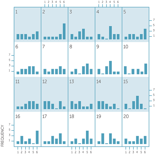
In some of the sets of 12 tosses, one of the numbers occurred up to 6 times, but in other sets, the frequencies were more even across the numbers. There is a lot of variation in what can be observed in 12 tosses of a die.
Below are 20 column graphs giving the frequencies of results in 24 tosses of a fair die.
Frequencies of results in 20 sets of 24 tosses of a die
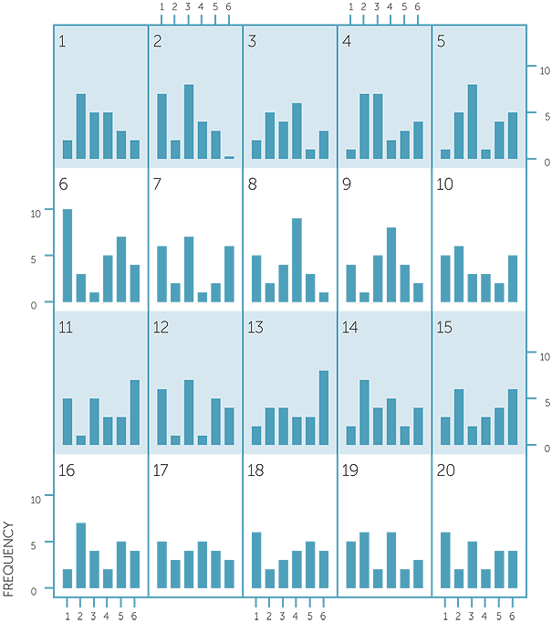
In one of the sets of 24 tosses, a number occurred 9 times, and in some there were frequencies of 7 or 8. Again there are other sets in which the frequencies are more evenly spread. However a frequency of 8 in 24 tosses is a relative frequency of  which corresponds to a frequency of 4 in 12 tosses. So a frequency of 6 occurrences out of
12 tosses is more extreme than a frequency of 8 or 9 in 24 tosses.
Below are column graphs of the frequency of the outcome of 6 in 12 tosses and in 24 tosses in both the above 20 sets − in the 20 sets of 12 tosses and in the 20 sets of 24 tosses.
Frequencies of 6'S in 20 sets EACH of 12 AND 24 tosses

Because there is a probability of  of getting a 6 in each toss, we would expect something like 2 tosses out of 12 giving us a 6, and something like 4 tosses out of 24 giving us a 6. So we see that although there was two sets of 24 tosses that gave as few 6’s as 0 or 1, and two that gave us as many as 7 or 8, there were many that gave 4 6’s. In contrast, as many sets of 12 tosses gave as 1 6 as those that gave 2 6’s and there tended to be a more variation in the number of 6’s we got in 12 tosses than in 24 tosses.
To demonstrate this further, the column graphs below give the frequencies of the outcome of 6 in 12 tosses and in 24 tosses of a fair die, repeated 50 times for each. Note that 2 was the most common number of 6’s in 12 tosses, and 4 the most common number of 6’s in 24 tosses, as we would expect. But we see that in 12 tosses, the number of 6’s ranged from 0 to 5, while in 24 tosses the number of 6’s ranged from 0 to 10.
Frequencies of 6'S in 50 sets EACH of 12 AND 24 tosses

Example C: Who gets the “prize”?
To simulate the drawing of a raffle with a person having a 10% chance of winning, a random number generator is needed to generate data from a set of probabilities of 0.1 and 0.9 each for “yes” and “no” respectively (or for the numbers 1 and 0 respectively). In a single draw, either a “yes” or a “no” card is the outcome. If we repeat the draw many times, we get some idea of what a 10% chance gives in real observations.
Frequencies of yes'S in 10, 20 and 50 draws,
simulated 50 times each

We see that often in 10 draws, we get no “yes” card. In 20 draws and in 50 draws, we would expect to get approximately 2 “yes” cards and 5 “yes” cards respectively. Although the simulated data shows that the number of “yes” cards obtained did tend to centre on what we would expect, there were many sets of draws that gave us fewer or more “yes” cards than we would expect.
The column graphs below use the same simulated data, but graph the relative frequencies of “yes” cards in 10, 20 and 50 draws, with each simulation repeated 50 times. These show how the relative frequencies become less varied around 0.1 the bigger the number of draws.
relatives Frequencies of yes'S in 10, 20 and 50 draws

The above simulations are just some examples of data that can be observed. If these simulations are repeated, different datasets will be obtained, and it is possible that some of the contrasts might be quite surprising. But the general features in the above simulations are fairly indicative of the effects of probabilities of  and
and  .
.
Note for teachers
Remember that we are only looking at overall frequencies and relative frequencies here. We are not looking at sequences of observations. Students need to feel confident that in successive throws of a die (whether real or simulated) or draws of a card from a container (replacing the card each time), the chances of the outcomes are the same, but we are not looking at sequences of outcomes, just overall frequencies and relative frequencies. This is particularly important to emphasize in looking at frequencies of letters in text or vocabulary as clearly some letters are more likely to follow a particular letter than others.
Some general comments and links
from F-5 and towards year 7
From Years 1−5, students have gradually developed understanding and familiarity with simple and familiar events involving chance, including possible outcomes and whether they are “likely”, “unlikely” with some being “certain” or “impossible”. They have seen variation in results of simple chance experiments. In Year 4, they have considered more carefully how to describe possible outcomes of simple situations involving games of chance or familiar everyday outcomes, and how the probabilities of possible outcomes could compare with each other. They have also considered simple everyday events that cannot happen together and, in comparison, some that can.
In Year 5, consideration of the possible outcomes and of the circumstances of simple situations has lead to careful description of the events and assumptions that permit assigning equal probabilities, understanding what the values of these probabilities must be and representing these values using fractions.
In Year 6, decimals and percentages have been used along with fractions to describe probabilities; this also helps to increase the sense of the size of probabilities and the extent − or lack of it − of the chance of outcomes. Understanding of probability has been extended to considering the implications for observing data in situations involving chance. Each time we observe a situation involving chance, only one possible outcome can be observed. The values of probabilities tell us the chance of observing each outcome each time we take an observation, but what can we expect to see in a set of observations? In Year 6 students have collected data and carried out simple simulations of data to experience the effects of chance on observations.
To use Excel to generate random data, requires the add-in of Data Analysis under Tools.
To use Data Analysis under Tools to simulate a number of random throws of a fair die requires the numbers 1 to 6 to be entered in a column, with the next column consisting of equal probabilities in each cell. As this second column must sum to 1, you might need to slightly adjust values you enter to ensure this; for example, 4 values could be 0.167 and 2 values 0.166. Choose Random Number Generator. In Number of Variables, enter the number of samples you wish to generate. In Number of Random Numbers, enter the size of the samples. For example, if you enter 1 in Number of Variables and 10 in Number of Random Numbers, you will simulate 10 throws of the die. If you enter 3 in Number of Variables and 10 in Number of Random Numbers, you will simulate 3 sets of 10 throws of the die. In Distribution, choose Discrete. In Value and Probability Input Range, give the column in which you placed the possible outcomes (for the die, this is 1 to 6), and the column in which each possible value is equal (allowing for perhaps a slight adjustment) and sum to 1. In Output Options, choose New Worksheet or, if Output Range, give a range of number of columns being the chosen number of samples, and the size of each column being the chosen sample size.
To use Data Analysis under Tools to simulate a number of draws of a raffle with a fixed constant chance of winning (instead of just simulating single draws at a time as in the above paragraph), involves generating a number of random samples of data on a categorical variable with a given probability for the category of interest. Choose Random Number Generator. For Number of Variables, enter 1. For Number of Random Numbers, enter the number of different samples you want to generate − for example, 50 simulations have been used in Example C above. For Distribution, choose Binomial.
Under the Parameters that appear for Binomial, the p Value is the probability of winning in just one draw of the raffle (10% in Example C above), and the Number of trials is the number of draws of the raffle you wish to simulate (In Example C above, 10, 20 and 50 draws were simulated). If you choose to use the output range, it needs to be a single column of the same size as the Random Number you chose. The output will consist of a set of numbers out of the Number of trials, so divide by the Number of trials to obtain the simulated relative frequencies.
Note for teachers’ background information.
Much is written in educational literature about coin tosses and much has been tried to be researched and analysed in students’ thinking about coin tossing. This situation is far more difficult than is usually assumed in such research which often tends to take the assumptions of fair coins and independent tosses as absolutely immutable and not to be questioned. In addition a common mistake is to state that it demonstrates either poor or, in contradiction, good thinking, to say that a particular sequence of coin tosses with a mixture of heads and tails is more likely than a sequence of the same outcome, when in practice it is not made clear whether the researcher or the student is thinking of a particular ordered sequence or merely a mixture of heads and tails. For example, if a coin is fair and tosses are independent, the chance of HTHHTT is EXACTLY the same as the chance of HHHHHH, but many people think of the first outcome in terms of getting 3 H’s and 3 T’s which is not the same as getting a particular sequence with 3 H’s and 3 T’s.
With regard to the assumption of a fair coin and independent tosses, the assumptions are the same as tossing dice. However, it is more difficult in practice to toss a coin completely randomly than to toss dice randomly, and also to assume that a particular person does not tend to toss a coin in a similar manner each toss. It is also extremely difficult in practice to identify whether unlikely sequences are due to an unfair coin or how it is tossed, and it would be of far greater benefit in research, but far more challenging, to devise experiments in which these two assumptions could be separately investigated.
Indeed, if, on observing an unlikely sequence, students do question either the fairness of a coin or no connection between consecutive coin tosses, then are they not demonstrating intuitive understanding of statistical hypothesis testing? Note that there is a difference between observing a simulation and observing a real situation because assumptions are easier to accept in a simulation.
For some excellent comments on this, see the letter by Harvey Goldstein to the Editor of Teaching Statistics (2010), Volume 32, number 3.
Because of the over-emphasis in educational research on coin tossing, and the problems caused by lack of clarity and understanding in much written on this topic, examples using coin tossing are avoided as much as possible in these modules.
The Improving Mathematics Education in Schools (TIMES) Project 2009-2011 was funded by the Australian Government Department of Education, Employment and Workplace Relations.
The views expressed here are those of the author and do not necessarily represent the views of the Australian Government Department of Education, Employment and Workplace Relations.
© The University of Melbourne on behalf of the International Centre of Excellence for Education in Mathematics (ICE-EM), the education division of the Australian Mathematical Sciences Institute (AMSI), 2010 (except where otherwise indicated). This work is licensed under the Creative Commons Attribution-NonCommercial-NoDerivs 3.0 Unported License.
https://creativecommons.org/licenses/by-nc-nd/3.0/
![]()