Content
Relative frequencies and continuous distributions
Continuous random variables are technically an abstraction (\(\Pr(X = x) = 0\)), and all variables that we measure are in practice, as measured, discrete. Even quantities that seem to be intrinsically continuous, like time, are always measured to the nearest unit of time, depending on the context. The following table illustrates this.
| Context | Smallest unit of time usually used |
|---|---|
| Cosmology | 10 million years (0.01 billion years) |
| Geological scale | MYA (million years ago) |
| Recorded history | year |
| Recent history | day |
| 'What's the time?' | minute |
| Jogger | second |
| Many sports (athletics, swimming, \ldots) | hundredth of a second |
| Formula 1 racing | thousandth of a second |
This discreteness follows from the rounding that occurs, either by necessity or by convention. There are many such examples in everyday life and also in research. We usually measure the height of individuals to the nearest centimetre, but it is easy to envisage a greater accuracy of measurement: to the nearest millimetre, for example.
Given all this intrinsic or necessary discreteness in measured variables, why not stick to the use of discrete distributions for modelling? Why use continuous distributions at all, especially if a continuous random variable is really an abstraction rather than a reality?
The answer is that it is often convenient and useful to use a continuous distribution, rather than attempting to use a discrete model.
Example: Train trips
Consider a study of a particular train trip in a timetable, from an outer suburban train station to a central city station. The purpose of the study is to check whether the actual times are adhering to the train timetable. The train's departure time and arrival time are recorded for 250 days. The times are measured to one-second accuracy, so that times such as 42 minutes and 7 seconds (42:07) are recorded.
The average time recorded, to the nearest second, was 2598 seconds (which corresponds to 43:18 minutes, or to 43.3 minutes as a decimal). The minimum time was 2466 seconds (41:06 minutes), and the maximum time was 3747 seconds (62:27 minutes).
If we regarded this random variable as being discrete, with possible values at every second (\(\dots, 2800, 2801, 2802, \dots\)), and sought to model it using a discrete distribution, we would need to come up with probabilities for each second separately. In the absence of a theoretical basis for doing so, we might consider using the gathered data to estimate these probabilities.
Think of the consequences of doing this. There are 1282 discrete times (to the nearest second) in the range of the data, from 2466 to 3747 seconds. With \(n=250\) observations, most of these discrete values will not appear in the data, that is, they will have a frequency of zero. Of the rest, most will have a count of one, some will have two, and a handful of the discrete values might have occurred three or more times in the data set.
It would therefore be quite cumbersome to model the times as discrete. It is convenient to think of the times as coming from an underlying theoretical distribution which is continuous. We can then look at the continuous distribution and its properties to understand more about the pattern of the train-trip times.
A related point is that it is unlikely that we would ever need to consider the lengths of the train trips at the detailed level of the individual discrete times. It is much more likely that we would be interested in, say, the percentage of trips between 42 and 43 minutes, or the fraction of trips that are five minutes late or worse, and so on, rather than the chance that a train trip is 43 minutes 30 seconds.
figure 10 shows a histogram of the 250 train trips. Alongside it is the pdf of a continuous random variable. This pdf is given by the following formula:
\[ f(x) = \dfrac{\exp\Bigl(-\dfrac{1}{2}\bigl[\ln(x-41) - 0.4\bigr]^2\Bigr)}{\sqrt{2\pi}(x-41)}, \qquad\text{for } x > 41. \]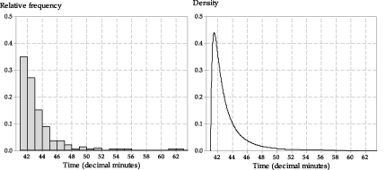
Figure 10: Comparison of relative-frequency data and a postulated model.
The relative frequencies in the histogram correspond to the areas under the graph of the probability density function. We can assess whether the model is a good fit to the data by looking at the probabilities from the pdf, and asking how close they are to the relative frequencies in the histogram.
For example, there were 87 trips between 41:00 minutes and 41:59 minutes; this is a relative frequency of \(\dfrac{87}{250} = 0.348\). How close is this to the probability implied by the pdf? Calculating the area under the graph of this pdf is beyond the curriculum, but it is found to be \(0.345\), which is very close to the relative frequency. The following table shows the relative frequencies and the corresponding probabilities from the pdf, for the first five one-minute intervals.
| Time interval (minutes) | Frequency | Relative frequency | Probability from model |
|---|---|---|---|
| 41:00 – 41:59 | 87 | 0.348 | 0.345 |
| 42:00 – 42:59 | 68 | 0.272 | 0.271 |
| 43:00 – 43:59 | 38 | 0.152 | 0.142 |
| 44:00 – 44:59 | 22 | 0.088 | 0.081 |
| 45:00 – 45:59 | 9 | 0.036 | 0.049 |
This example illustrates the way that continuous distributions are often used: as a useful approximation to a discrete random variable, when the discrete random variable is on a very fine scale. This occurs in a wide variety of contexts, such as measurements of human heights (centimetres), IQ (integers), exam marks and so on.
In circumstances where we do not have a clear basis for choosing a particular pdf to model data of this sort, the relative frequencies from the histogram serve as a guide: we obtain estimates of probabilities for given intervals directly. We then look for a continuous distribution that can closely reflect these estimates.
In the module Exponential and normal distributions , we will see this in practice; the data being considered are measured on a fine discrete scale, but are modelled using a continuous distribution.
Example: Taxi fares
exercise 6 involves taxi fares. Any actual taxi fare is in dollars and cents, and hence the variable 'taxi fare' is discrete: it only takes values to the nearest five cents. To model the variation in taxi fares, however, we would typically use a continuous distribution.
Next page - Answers to exercises
| This publication is funded by the Australian Government Department of Education, Employment and Workplace Relations |
Contributors Term of use |