Answers to exercises

Exercise 1

1. On the interval \([0,1]\), the function \(f(x)\) is a quadratic with a negative coefficient of \(x^2\) and \(x\)-intercepts 0 and 1. Thus \(f(x) \geq 0\), for \(x\) in \([0,1]\). By definition, we have \(f(x) = 0\), for \(x\) outside the interval \([0,1]\). Hence, the first property is satisfied: \(f(x) \geq 0\), for all \(x\).
   
   To check the second property, we calculate: \begin{align*} \int_{-\infty}^{\infty} f(x)\;dx &= \int_0^1 6x(1-x)\;dx \\\\ &= \int_0^1 6x - 6x^2\;dx \\\\ &= \bigl[3x^2 - 2x^3\bigr]^1_0 \\\\ &= 1. \end{align*} So the second property is also satisfied.
   
   The graph of \(f(x)\) is shown in the following figure.
   
   
   
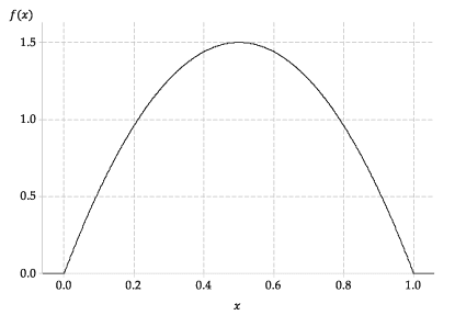
   Figure 11: The probability density function \(f(x)\).
2. By considering the function or the graph, it is clear that:
   1. \(\Pr(X \leq -3) = 0\)
   2. \(\Pr(0 \leq X \leq 1) = 1\)
   3. \(\Pr(0.5 \leq X \leq 1) = 0.5\), since the pdf is symmetric about \(x = \dfrac{1}{2}\).
3. To guess this probability, you need to estimate the area under the curve between 0.4 and 0.7. You can do this subjectively, keeping in mind that the total area under the curve is 1. Using the gridlines in figure 11 as a guide, we can make a slightly more informed guess:

• The area under the curve between 0.4 and 0.6 is nearly \(0.2 \times 1.5 = 0.3\).
• The region under the curve between 0.6 and 0.7 is a rectangle of area \(0.1 \times 1 = 0.1\) plus a small region whose area appears to be a bit less than \(\dfrac{3}{4} \times 0.1 \times 0.5 = 0.0375\).

1. 1. \(f(0.2) = 0.96\), \(f(0.4) = 1.44\), so \(\lambda = \dfrac{1.44}{0.96} = 1.5\).
   2. \(p_{0.2} = \Pr(0.15 \leq X \leq 0.25) = \displaystyle\int_{0.15}^{0.25} 6x(1-x)\;dx = 0.0955\).
   3. \(p_{0.4} = \Pr(0.35 \leq X \leq 0.45) = \displaystyle\int_{0.35}^{0.45} 6x(1-x)\;dx = 0.1435\).
   4. \(\dfrac{p_{0.4}}{p_{0.2}} = \dfrac{0.1435}{0.0955} = 1.503 \approx \lambda\).

Exercise 2

1. By inspection of the graph in figure 7, we can see that \(f_V(v) \geq 0\), for all \(v\), and that the total area under the curve is \(\dfrac{1}{2} \times 1 \times 2 = 1\). Hence, the function has the two properties of a pdf.
2. The function \(f_V(v)\) is made up of two lines. Formally: \[ f_V(v) = \begin{cases} 4v &\text{if } 0 \leq v \leq \dfrac{1}{2}, \\\\ 4 - 4v &\text{if } \dfrac{1}{2} < v \leq 1, \\\\ 0 &\text{otherwise.} \end{cases} \]
3. For \(v > 0\), we have \(F_V(v) = \displaystyle\int_{0}^{v} f_V(t)\;dt\). We need to deal with the two parts of the pdf separately. For \(0 < v \leq \dfrac{1}{2}\), we have \[ F_V(v) = \int_{0}^{v} 4t\;dt = 2v^2. \] For \(\dfrac{1}{2} < v \leq 1\), we have \[ F_V(v) = \Pr(V \leq v) = \Pr(V \leq \tfrac{1}{2}) + \Pr(\tfrac{1}{2} < V \leq v), \] and so \begin{align*} F_V(v) &= \tfrac{1}{2} + \int_{0.5}^{v} (4-4t)\;dt \\\\ &= \tfrac{1}{2} + \bigl[4t - 2t^2\bigr]^{v}_{0.5} \\\\ &= \tfrac{1}{2} + (4v - 2v^2) - \tfrac{3}{2} \\\\ &= 4v - 2v^2 - 1. \end{align*} Putting these two parts together, we can write, formally, that the cdf of \(V\) is given by \[ F_V(v) = \begin{cases} 0 &\text{if } v \leq 0, \\\\ 2v^2 &\text{if } 0 < v \leq \dfrac{1}{2}, \\\\ 4v - 2v^2 - 1 &\text{if } \dfrac{1}{2} < v \leq 1, \\\\ 1 &\text{if } v > 1. \end{cases} \]
4. \(\Pr(0.2 \leq V \leq 0.3) = F_V(0.3) - F_V(0.2) = 0.1\). This can also be found from the pdf using the area of a trapezium.
5. We have \(f_V(0.3) = 1.2 > 0.8 = f_V(0.8)\), and so \(V \approx 0.3\) is more likely than \(V \approx 0.8\). (Here we write \(V \approx v\) to mean that \(V\) lies in a small interval of given width around \(v\).)

Exercise 3

1. For the first pdf: \[ f(x) = \begin{cases} \dfrac{1}{5}x &\text{if } 0 \leq x \leq 1, \\\\ \dfrac{1}{45}(10 - x) &\text{if } 1 < x \leq 10, \\\\ 0 &\text{otherwise.} \end{cases} \] For the second pdf: \[ f(y) = \begin{cases} \dfrac{1}{20}y &\text{if } 0 \leq y \leq 4, \\\\ \dfrac{1}{30}(10 - y) &\text{if } 4 < y \leq 10, \\\\ 0 &\text{otherwise.} \end{cases} \]
2. You need to guess where the centre of gravity of the pdf is, that is, where you would need to put the pivot to make the pdf balance. Reasonable guesses would be 'between 3 and 4' for the first pdf, and 'between 4 and 5' for the second pdf.
   
   If the continuous random variable \(X\) has the first pdf, then \begin{align*} \mathrm{E}(X) &= \int_{-\infty}^{\infty} x\,f(x)\;dx \\\\ &= \int_0^1 \dfrac{1}{5}x^2\;dx + \int_1^{10} \dfrac{1}{45}\bigl(10x - x^2\bigr)\;dx \\\\ &= \Bigl[ \dfrac{1}{15}x^3 \Bigr]_0^1 + \dfrac{1}{45}\Bigl[ 5x^2 - \dfrac{1}{3}x^3 \Bigr]_1^{10} \\\\ &= \Bigl( \dfrac{1}{15} - 0 \Bigr) + \dfrac{1}{45}\Bigl( \Bigl(500 - \dfrac{1000}{3} \Bigr) - \Bigl(5 - \dfrac{1}{3} \Bigr) \Bigr) \\\\ &= \dfrac{1}{15} + \dfrac{162}{45} = \dfrac{11}{3}. \end{align*} If the continuous random variable \(Y\) has the second pdf, then \begin{align*} \mathrm{E}(Y) &= \int_{-\infty}^{\infty} y\,f(y)\;dy \\\\ &= \int_0^4\dfrac{1}{20}y^2\;dy + \int_4^{10} \dfrac{1}{30}\bigl(10y - y^2\bigr)\;dy \\\\ &= \Bigl[ \dfrac{1}{60}y^3 \Bigr]_0^4 + \dfrac{1}{30}\Bigl[ 5y^2 - \dfrac{1}{3}y^3 \Bigr]_4^{10} \\\\ &= \Bigl( \dfrac{64}{60} - 0 \Bigr) + \dfrac{1}{30}\Bigl( \Bigl(500 - \dfrac{1000}{3} \Bigr) - \Bigl(80 - \dfrac{64}{3} \Bigr) \Bigr) \\\\ &= \dfrac{32}{30} + \dfrac{108}{30} = \dfrac{14}{3}. \end{align*}
3. The total area under the curve is 1. Reasonable guesses might be 'about a quarter' and 'a bit more than one half'. The values are \(\dfrac{2}{9} = 0.222\) and \(\dfrac{5}{8} = 0.625\), obtained by either integration or simple calculations of areas.

Exercise 4

1. The pdf of \(U\) is given by \[ f_U(u) = \begin{cases} 1 &\text{if } 0 \leq u \leq 1, \\\\ 0 &\text{otherwise.} \end{cases} \] We know the mean of the distribution is \(\mu_{U} = \dfrac{1}{2}\). First we find the variance: \begin{align*} \mathrm{var}(U) &= \int_{-\infty}^{\infty} (u - \mu_U)^2 f_U(u)\;du \\\\ &= \int_{-\infty}^{\infty} \Bigl(u - \dfrac{1}{2}\Bigr)^2 f_U(u)\;du \\\\ &= \int_0^1 \Bigl(u - \dfrac{1}{2}\Bigr)^2\;du \\\\ &= \int_0^1 \Bigl(u^2 - u + \dfrac{1}{4}\Bigr)\;du \\\\ &= \Bigl[ \dfrac{1}{3}u^3 - \dfrac{1}{2}u^2 + \dfrac{1}{4}u \Bigr]_0^1 \\\\ &= \dfrac{1}{3} - \dfrac{1}{2} + \dfrac{1}{4} = \dfrac{1}{12}. \end{align*} Hence, the standard deviation of \(U\) is \(\mathrm{sd}(U) = \sqrt{\dfrac{1}{12}} = 0.289\).
2. The pdf of \(V\) is given by \[ f_V(v) = \begin{cases} 4v &\text{if } 0 \leq v \leq \dfrac{1}{2}, \\\\ 4 - 4v &\text{if } \dfrac{1}{2} < v \leq 1, \\\\ 0 &\text{otherwise.} \end{cases} \] We know the mean of the distribution is \(\mu_V = \dfrac{1}{2}\). First we find the variance: \begin{align*} \mathrm{var}(V) &= \int_{-\infty}^{\infty} (v - \mu_V)^2 f_V(v)\;dv \\\\ &= \int_{-\infty}^{\infty} \Bigl(v - \dfrac{1}{2}\Bigr)^2 f_V(v)\;dv \\\\ &= \int_0^{\dfrac{1}{2}} \Bigl(v - \dfrac{1}{2}\Bigr)^2 4v\;dv + \int_{\dfrac{1}{2}}^1 \Bigl(v - \dfrac{1}{2}\Bigr)^2 \bigl(4-4v\bigr)\;dv \\\\ &= \int_0^{\dfrac{1}{2}} \Bigl(4v^3 - 4v^2 + v\Bigr)\;dv + \int_{\dfrac{1}{2}}^1 \Bigl(-4v^3 + 8v^2 -5v + 1\Bigr)\;dv \\\\ &= \Bigl[ v^4 - \dfrac{4}{3}v^3 + \dfrac{1}{2}v^2 \Bigr]_0^{\dfrac{1}{2}} + \Bigl[ -v^4 + \dfrac{8}{3}v^3 - \dfrac{5}{2}v^2 + v \Bigr]_{\dfrac{1}{2}}^1 \\\\ &= \Bigl(\dfrac{1}{16} - \dfrac{1}{6} + \dfrac{1}{8}\Bigr) - 0 + \Bigl(-1 + \dfrac{8}{3} - \dfrac{5}{2} + 1\Bigr) - \Bigl(-\dfrac{1}{16} + \dfrac{1}{3} - \dfrac{5}{8} + \dfrac{1}{2}\Bigr) = \dfrac{1}{24}. \end{align*} Hence, the standard deviation of \(V\) is \(\mathrm{sd}(V) = \sqrt{\dfrac{1}{24}} = 0.204\).

Exercise 5

From the previous exercise, we have \(\mu_V = 0.5\) and \(\sigma_V = 0.204\). Thus

\begin{align*} \Pr\bigl(\mu_V - 2\sigma_V \leq V \leq \mu_V + 2\sigma_V\bigr) &= \Pr\bigl(0.5 - (2 \times 0.204) \leq V \leq 0.5 + (2 \times 0.204)\bigr) \\\\ &= 2 \times \Pr(0.5 - 0.408 \leq V \leq 0.5), \end{align*}

because the pdf is symmetric about 0.5. Now

\begin{align*} \Pr(0.5 - 0.408 \leq V \leq 0.5) &= \Pr(0.092 \leq V \leq 0.5) \\\\ &= \int_{0.092}^{0.5} 4v\;dv \\\\ &= \bigl[ 2v^2 \bigr]_{0.092}^{0.5} \\\\ &= 0.5 - 0.0169 \\\\ &= 0.483. \end{align*}

Hence, \(\Pr\bigl(\mu_V - 2\sigma_V \leq V \leq \mu_V + 2\sigma_V\bigr) = 2 \times 0.483 = 0.966\). This is reasonably close to the probability 0.95 indicated by the rule of thumb.

Exercise 6

We have \(Y = 2.20 X + 3.20\).

Recall that \(\mathrm{E}(aX+b) = a\,\mathrm{E}(X) + b\). As \(\mathrm{E}(X) = 15\), this gives \(\mathrm{E}(Y) = 2.20 \times 15 + 3.20 = 36.20\). The average cost is $36.20.

Recall that \(\mathrm{sd}(aX+b) = |a|\,\mathrm{sd}(X)\). Since \(\mathrm{sd}(X) = 50\), this gives \(\mathrm{sd}(Y) = 2.20 \times 50 = 110\). The standard deviation of the cost is $110.