Answers to exercises

Exercise 1

As the distribution of the weight gain is assumed to be Normal, the distribution of the sample mean, \(\bar{X}\), is also Normal, and, specifically, \(\bar{X} \stackrel{\mathrm{d}}{=} \mbox{N}(\mu,\tfrac{4^2}{n})\). We want the probability that \(\bar{X}\) is within 1 kg of \(\mu\), or, equivalently, the chance that \(\bar{X}\) is betweeen \(\mu -1\) and \(\mu +1\). That is, we want \(\Pr(\mu - 1 < \bar{X} < \mu +1)\). We use the standardising steps to obtain the result:

\begin{eqnarray*} \Pr(\mu - 1 < \bar{X} < \mu +1) & = & \Pr( - 1 < \bar{X} - \mu < 1) \quad \quad \quad \quad \quad \quad \mbox{(subtracting \(\mu\) throughout)}\\ & = & \Pr\left(\frac{-1}{4/\sqrt{n}} < \frac{\bar{X} - \mu}{4/\sqrt{n}} < \frac{1}{4/\sqrt{n}}\right) \quad \quad \mbox{(dividing through by \(4/\sqrt{n}\))}\\ & = & \Pr\left(\frac{-1}{4/\sqrt{n}} < Z < \frac{1}{4/\sqrt{n}}\right) \quad \quad \quad \quad \mbox{(where \(Z \stackrel{\mathrm{d}}{=}\) N(0,1)).}\\ \end{eqnarray*}

Using calculators or software, the probabilities are:

\(n = 5: \Pr(-0.5590 < Z < 0.5590) = 0.4238.\)
\(n = 20: \Pr(-1.1180 < Z < 1.1180) = 0.7364.\)
\(n = 50: \Pr(-1.7678 < Z < 1.7678) = 0.9229.\)

What does this mean in practice? From a random sample of \(n=5\), there is only a 42% chance that the sample mean is within 1 kg of the true mean \(\mu\). By increasing the sample size to 50, this becomes about 92%, much higher.

Exercise 2

For each value of \(\bar{x}_{\mbox{obs}}\) considered, we need to find \(\Pr\left(|\bar{X} - 95| \geq |\bar{x}_{\mbox{obs}} - 95|\right).\)

For \(\bar{x}_{\mbox{obs}} = 94.9\), we obtain the following: \begin{eqnarray*} \Pr(|\bar{X} - 95| \geq |94.9 - 95|) & = & \Pr(|\bar{X} - 95| \geq 0.1)\\ & = & \Pr\left(\left|\frac{\bar{X} - 95}{1.2/5}\right| \geq \frac{0.1}{1.2/5}\right) \quad \quad \mbox{(standardising)}\\ & = & \Pr(|Z| > 0.4167) \quad \quad \quad \quad \mbox{(where \(Z \stackrel{\mathrm{d}}{=}\) N(0,1))}\\ & = & 0.6722. \end{eqnarray*}
0.0956
0.0009

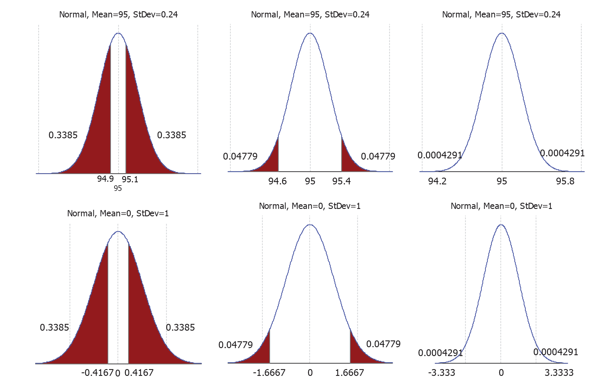
Figure 3: Distribution of the sample mean for Exercise 2, \(\bar{X}\), shown in top row; corresponding distribution of the standard Normal, Z, in the bottom row. Probabilities for (a), (b) and (c) from left to right.

The probabilities required in each case correspond to the total of the two shaded areas in Figure 3. The two areas are equal, by symmetry, and the numbers shown on the probability density functions are the (equal) probabilities of each of these areas. For example, for (c), \(\Pr(|Z|>3.3333) = \Pr(Z < -3.3333) + \Pr(Z > 3.3333) = 0.0004291 + 0.0004291 = 0.0009\) (to four decimal places).

These answers confirm the visual impression gained from Figure 1. An observed sample mean of 94.9 g from a random sample of 25 cans is not unusual, while \(\bar{x} = 95.4\) is slightly unusual. However, \(\bar{x} = 94.2\) is very unusual indeed: samples such as this would occur only 9 times in 10,000 (in a repeated sampling sense).

Exercise 3

For the given context, \(Z = \frac{\bar{X} - \mu_0}{\sigma/\sqrt{n}} \stackrel{\mathrm{d}}{=} N(0,1)\) if the null hypothesis \(\mu = \mu_0\) is true. If \(P \geq 0.05\) for testing this null hypothesis, then \(|z| \leq 1.96\).

\begin{eqnarray*} |z| \leq 1.96 & \Rightarrow & \left|\frac{\bar{x} - \mu_0}{\sigma/\sqrt{n}}\right| \leq 1.96\\ & \Rightarrow & |\bar{x} - \mu_0| \leq 1.96 \frac{\sigma}{\sqrt{n}}\\ & \Rightarrow & \bar{x} - 1.96 \frac{\sigma}{\sqrt{n}} \leq \mu_0 \leq \bar{x} + 1.96 \frac{\sigma}{\sqrt{n}} \end{eqnarray*}

Since the 95% confidence interval is \((\bar{x} - 1.96 \frac{\sigma}{\sqrt{n}}, \bar{x} + 1.96 \frac{\sigma}{\sqrt{n}})\), it follows that \(\mu_0\) is in this interval.

Further, the implications in this argument are all "if and only if", so the result applies in reverse. If a particular value of \(\mu\), \(\mu_0\), say, is in the 95% confidence interval for \(\mu\), then the \(P\)-value for testing \(\mu = \mu_0\) must be at least 0.05.

Exercise 4

The probability that the average electronic media use of 11-year olds meets the Government recommendations is 0.001.
This statement is incorrect; the \(P\)-value is not the probability that the null hypothesis is true.
The probability that the study is wrong is very small.
This statement is incorrect; the \(P\)-value does not provide information about whether the results are right or wrong.
The average electronic media use of 11-year olds is estimated to be more than one hour above the Government recommendation. This is a correct statement about the observed mean number of hours of electronic media use.
The result is not consistent with the Government recommendation, as \(P = 0.001\).
This is a correct statement about the \(P\)-value.
The confidence interval suggests that average electronic media use of 11-year olds could be between 0.5 and 1.7 hours above the recommendation.
This statement provides an appropriate interpretation of the bounds of the confidence interval.

Exercise 5

The large \(P\)-value shows that average electronic media use of 6-year olds meets the Government recommendations.
This statement is vague; large \(P\)-values do not mean that the null hypothesis is true.
The average electronic media use of 6-year olds is estimated to be half an hour above the Government recommendation.
This is a correct statement about the observed mean number of hours of electronic media use.
The result is consistent with the Government recommendation, as \(P = 0.18\).
This is a correct statement about the \(P\)-value.
The confidence interval suggests that average electronic media use of 6-year olds could be as much as 1.2 hours above the recommendation.
This statement provides an appropriate interpretation of the upper bound of the confidence interval.
The Government need not be concerned about the electronic media use of 6-year olds as the \(P\)-value is 0.18.
This statement is ambiguous. It could be interpreted as implying that the null hypothesis is true because the \(P\)-value is large; this is incorrect. The \(P\)-value does not tell us about the 'truth' of the null hypothesis.