The Improving Mathematics Education in Schools (TIMES) Project

return to index

The Real Numbers

Number and Algebra : Module 28Years : 8-10

June 2011

PDF Version of module

Assumed Knowledge

• Fluency with integer arithmetic.
• Familiarity with fractions and decimals.
• Facility with converting fractions to decimals and vice versa.
• Familiarity with Pythagoras’ Theorem.

Motivation

This module differs from most of the other modules, since it is not designed to summarise in one document the content of material for one given topic or year. Material related to the real numbers is scattered throughout the modules. We felt, however, that it was important to have a short module on the real numbers to bring together some of the important ideas that arise in school mathematics.

From the beginning of their mathematical studies, students are introduced to the whole numbers. Later, fractions and decimals are introduced, leading to the notion of a rational number, then the integers and negative fractions and decimals are covered. Finally the notion of real number is gradually introduced after Pythagoras’ theorem has been covered.

Throughout this module we will use the term rational numbers for positive and negative fractions including the integers. The rational numbers are numbers of the form where m is an in integer and n a non-zero integer. An irrational number is a number which is not rational.

The integers and rational numbers arise naturally from the ideas of arithmetic. The real numbers essentially arise from geometry. Finding the length of the diagonal of a square leads to square roots of numbers that are not squares. When we draw a circle whose radius is a whole number and ask for its diameter and area, the answer involves the irrational number π.

It was as a consequence of Pythagoras’ theorem that the Greeks discovered irrational numbers, which shook their understanding of number to its foundations. They also realised that several of their geometric proofs were no longer valid. The Greek mathematician Eudoxus considered this problem (see the History section), and mathematicians remained unsettled by irrational numbers for a very long time. The modern understanding of real number only began to be developed during the 19th century.

It is not possible to give a rigorous treatment of real numbers at high school. Nonetheless, we can give a reasonable answer to the student who asks `What is a real number?’ and we can also explain why such numbers are important.

Content

Rational Numbers

A rational number is one that can be expressed in the form where p is an integer, and q is a non-zero whole number. Fractions, terminating and recurring decimals are all examples of rational numbers.

Thus: 5 = , −3 = , 2 = , −6.19 = , 20% =

are all examples of rational numbers.

In the module, Integers, we showed, in an appendix, how the integers could be constructed from the whole numbers using ordered pairs. In the first Appendix to
this module we show how the rational numbers can be constructed in a similar way.
This is needed to cope with the multiple representation of a fraction. For example, = .

You will have seen in the module, Decimals and Percentages. That every fraction can be expressed as either:

• a terminating decimal, for example, = 0.625, or
• a recurring decimal, for example, = 0.8571, and = 0.1 where the dots indicate repetition.

A fraction, , in reduced form where p and q are whole numbers with no common factors, will have a terminating decimal representation if and only if q has no prime factors except 2 and 5.

All fractions can be converted to a decimal by using long division. This involves dividing the denominator into the numerator. A zero remainder at some stage in the division will result in a terminating decimal. If the remainder is never zero, then division by a denominator q will result in a repeating pattern of remainders after at most (q − 1) steps (see the module, Decimals and Percentages).

Decimals to Fractions

The technique for converting decimals to fractions depends on whether the decimal is terminating, recurring or eventually recurring. A terminating decimal can be easily converted back to a fraction by using a denominator which is a power of 10.

For example, 3.14 = 3 + = 3 + = .

The following example demonstrates the method for converting recurring
decimals to fractions.

An eventually recurring decimal can easily be handled by firstly multiplying it by a sufficiently high power of 10 to make its decimal part purely recurring.

Paradise Lost

We first prove the following result about fractions:

‘If a fraction is not a whole number, then its square is not a whole number either.’

Proof

Suppose that is in reduced form, so that a and b have no common factors except 1. Then a2 and b2 also have no common factors, because if any prime p were a common factor of a2 and b2, it would also be a common factor of a and b.
Hence is not a whole number.

Since is not a whole number, but its square is the whole number 2, it follows from the above result that is not a rational.

This caused great upset to the Greek mathematicians, since it introduced a new sort of number which they called an irrational number. An older word for this is incommensurable, which meant that it could not be measured as a ratio of two whole numbers. This discovery caused a dramatic rethink into the nature of number. The validity of many of their geometric proofs, which assumed that all lengths could be measured as ratios of whole numbers, was also called into question.

The proof given above can easily be adapted to prove that if a whole number x is not an nth power, then is not a rational number. Thus we have infinitely many examples of irrational numbers, such as:

, ,

Such numbers are called surds and will be discussed in detail in the module, Surds.

In addition, numbers such as π, log10 3, log2 6, sin 22°, and so on, are also irrational, although it is harder to prove this fact for the first and last of these examples. There is no general method for telling when a number is irrational, and indeed there are numbers such as π + e that arise in mathematics whose status is currently unknown.

The Fundamental Theorem of Arithmetic (The module, Prime and Prime Factorisation) can be used to generalize this result.

The real numbers

Think about graphing the rational numbers between 0 and 2 on the number line. First we graph , 1, then the thirds, then the quarters, then the fifths, …. As we keep going, the gaps between the dots get smaller and smaller, and as we graph more and more rational numbers, the largest gap between successive dots tends to zero.

If we imagine the situation when all the infinitely many rational numbers have been graphed, there appears to be no gaps at all, and the rational numbers are spread out like pieces of dust along the number line. Surely every point on the number line has been accounted for by some rational number?

Not true! There are infinitely many numbers that we have not graphed, all rational multiples of , including:

Of course, there are many more missing numbers, like and log2 3 and . We need a new definition of ‘numbers’ that will cover all these irrational objects, which are not rational numbers, but which we nevertheless want to think of as numbers. The solution is very simple — we make an appeal to geometry and define numbers using the geometrical idea of points on a line:

Definition The real numbers are all of the points on the number line.

The set of real numbers consists of both the rational numbers and the irrational numbers.

Constructing real numbers

We have seen in the module Constructions that every rational number can be plotted on the number line. For example, to plot we first divide the interval from 0 to 1 into 5 equal
subinterval (this requires the construction of

Thus rational numbers are indeed special cases of real numbers.

We also saw how to place the square root of any whole number on the number line using Pythagoras’
theorem. For example, to plot we first construct a
square on the interval from 0 to 1 (the constructions
of the right angles are not shown on the diagram).
Then we draw the diagonal from 0, which has
length , and use compasses to place this length
on the number line.

The real numbers and the rational numbers

We have seen that as we place halves, thirds, quarters, fifths, … on the number line, the maximum gap between successive fractions tends to zero. Thus if α is any real number then rational numbers will be placed increasingly close to α. Thus we can use rational numbers to approximate a real number correct to any required order of accuracy.

For example, the diagrams above show a circle of area π enclosed in a square of area 4, and enclosing a square of area 2, which proves that 2 < π < 4. Archimedes improved greatly on this result by using regular polygons with 96 sides, and was able to prove that 3 < π < 3.

Modern computer calculations, and the extremely clever algorithms they are based on, give approximations to π up to a trillion decimal places.

But beware! These observations might lead one to believe naively that the rational and irrational numbers somehow alternate on the number line. Nothing could be further from the truth. Even though there are infinitely many rational numbers and infinitely many irrational numbers between 0 and 1, there are vastly more real numbers in that interval than rational numbers.

This spectacular, but rather vague, claim can be made into a theorem as precise as any other mathematics, and proven rigorously — see the Appendix 2 for the details, which are an excellent challenge for interested and able students. Intuitively, one should see the real number line as a continuum, with the points joined up to make a line, whereas the rational numbers are like disconnected specks of dust scattered along it.

The real numbers and decimals

We have seen that every rational number can be written as a terminating or recurring decimal. Conversely, every terminating or recurring decimal can be written as a fraction, and thus as a rational number. Now suppose that we have a decimal that is neither terminating nor recurring, such as 1.01001000100001 …. where the number of zeroes increases by 1 each time. This decimal represents a definite point on the number line, and so is a real number, but it is not a rational number, because it neither terminates nor recurs. Indeed, any infinite decimal that is neither terminating nor recurring represents an irrational real number, and two different such infinite decimals represent different real numbers.

Now suppose that α is an irrational real number between 0 and 1. As we add tenths, hundredths, thousandths, ..to the number line between 0 and 1, the gap between adjacent dots decreases to zero.

By placing α successively between the tenths, between the hundredths, between the thousandths, we can produce an infinite decimal expansion that represents α. The conclusion of all this is the following theorem.

‘Every real number can be represented by one, and only one, infinite decimal (excluding recurring nines). If the expansion terminates or recurs, the number is rational, otherwise the number is irrational.’

Approximating real numbers by decimals

There are many ways of approximating real number by decimals. The two simplest are described below.

Sequence of truncations

Now consider the infinite decimal expansion of a real number α If we truncate this expansion at 1 place, 2 places, 3 places, …, the result is a sequence of rational numbers (terminating decimals) converging to α. For example, the decimal expansion of π is known to nearly 3 trillion places, and begins

π = 3.141592653589793238462643383279502884197169399375…

so the sequence of truncations begins

3.1, 3.14, 3.141, 3.1415, 3.14159, 3.141592, 3.1415926, 3.14159265, …

Sequence of approximations

To approximate the real number to a given number of decimal places, we truncate it one place more and then round in the usual way. Thus the sequence of approximations to π are

3.1, 3.14, 3.142, 3.1416, 3.14159, 3.141593, 3.1415927, 3.14159265, …

Of course this procedure can be applied just as easily to a recurring decimal, or to an overlong terminating decimal. This method of approximating real numbers by terminating decimals of whatever length is required is one reason why decimal expansions are so useful in science and everywhere that mathematics is applied.

Arithmetic with real numbers — using approximations

Having defined real numbers as points on the number line, how are we to define addition, subtraction, multiplication and division of real numbers? The most obvious approach is to work with their decimal expansions, and add, subtract, multiply and divide suitable truncations of these expansions. For example, suppose we want to add, subtract, multiply and divide π and correct to two decimal places.

We obtain correct to two decimal places

π + ≈ 4.56, π − ≈ 1.73, π × ≈ 4.44, π ÷ ≈ 2.22,

For people such as calculator and computer programmers who are concerned with the accuracy of such calculations, there are serious problems here about the number of decimal places necessary in the calculations and the sizes of possible errors, but these things need not concern us here.

It is, however, worth commenting on the infinitely recurring 9s that result from attempting non- truncated calculations such as

We know that both answers are 1, because + = 1 and × 3 = 1

In the module, Decimals and Percentages we defined 0. = 1. To justify this, we remarked that if 0. represents a number x, then 1 − x is a non-negative number less than every positive number, so 1 − x = 0. Similarly, any decimal expansion with an infinite string of 9s can always be replaced by a terminating decimal.

Arithmetic with real numbers — using geometry

Since real numbers have been defined geometrically, we should be able to describe the operations of arithmetic with real numbers using geometry alone. Addition and subtraction are straightforward. We can construct the sum a + b of two real numbers a and b in the usual way. We draw a straight line and on it mark off with a compass the distances OA = a and AB = b. Then OB = a + b. Similarly for a − b we mark of OA = a and AB = b but this time with AB in the opposite direction to OA. Then OB = a − b.

The opposite of a real number can be constructed as its reflection in the origin (using compasses). Multiplication and division require similarity. We have taken the similarity tests as axioms of our geometry, and we now can construct multiplication and division of real numbers on the number line in terms of the ratios and products of lengths introduced in the theory of similarity. The following exercise shows how to construct the product ab, the quotient a ÷ b and the reciprocal on a number line, where a and b are positive real numbers. Reflection in the origin then extends these constructions to negative real numbers.

In an earlier exercise you proved that between any two rational numbers there is a rational number. The following exercise shows that between any two rational numbers there is an irrational number.

It is also possible to show that between any two irrationals there is a rational number.
This is harder and is left to the Links Forward section.

The Real Numbers and Algebra

Numbers other than rational number frequently occur in problems involving measurement, areas and volumes, where the number π often makes an appearance. Quadratic surds also arise quite naturally when we find heights and sides of triangles. A quadratic surd involves the square root of a non-square whole number. Irrational numbers also arise in trigonometry since the sine, cosine and tangent ratios of most angles are irrational. We usually approximate these numbers using a calculator. Certain special angles have quadratic surds as their sine, cosine or tangent ratios.

For example, cos 30° = , sin 45° = .

Irrational numbers also arise when we solve equations of degree greater than one. Thus, the real solution of x3 = 5 is x = .

Quadratic surds often arise when we solve quadratic equations using either the method of completing the square or the quadratic formula.

When performing calculations, it is best to leave real numbers in exact form, at least until the end of a problem. We can then, if required, find approximate values. Converting real numbers to decimal approximations can lead to cumulative rounding errors.

Links Forward

Sequences

We can approximate all irrational numbers by rational numbers. This is often done by means of sequences.

Define the sequence a1, a2, … by a1 = 1 and for n > 1 = an + 1 =

Substituting in successive values, we obtain

a1 =1 , a2 = 1.5, a3 =1.416666… , a4 = 1.4142156…, and so on.

These numbers appear to be getting closer to the decimal 1.41421… which is the beginning of the decimal expansion for . If we assume that this sequence converges to some real number that is, we assume that the terms of the sequence approach α as grows without bound. As n gets bigger and an + 1 gets closer to an a good idea of what α should be can be found by replacing an and an + 1 in the equation above by α and we have

which simplifies to, α2 = 2. So α = since α is positive. Thus we have a sequence of rational numbers which converge to the real number .

Approximations to many real numbers can be obtained in this way.

Rationals between irrationals

We have seen that

• between any two rational numbers there is a rational number
• between any two rational numbers there is an irrational number.

It is also possible to show that

• between any two irrational numbers there is a rational number
• between any two irrational numbers there is an irrational number.

Here is a proof of the third dot point.

Proof

Suppose we take two irrational numbers, which we may as well assume are positive, where α < β.

We imagine that these two numbers are very close to each other, (although the proof works the same if they are not), so that the number δ = β − α is small.

Now no matter how small δ is, we can always multiply it by a whole number n to make the product greater than 2.

(For example, if δ = 0.00003145..., then we take n = 60 000 say, then nδ ≈ 2.07 > 2.)

Now look at the numbers na, nb. The distance between these numbers is

nβ − nα = n(β − α) = nδ > 2.

Since there is a gap of at least 2 between these numbers, then there is at least one whole number m, between them. That is,

nα < m < nβ.

Dividing by n we have,

α < < β.

Since m and n are whole numbers, we have constructed a rational number between the two given irrational numbers.

Continued Fractions

A continued fraction is an expression with either a finite or infinite number of steps

such as 2 + .

If we truncate the continued fraction somewhere, it can be simplified to produce a rational number. For example,

2 + = 2 + = 2 + = 2 + = .

The continued fraction given here is usually represented using the notation [2; 3, 5, 7].

It is easy to see that a rational number has a finite continued fraction. Therefore continued fractions that continue indefinitely represent irrational numbers. Continued fractions that repeat, such as [1; 2, 2, 2, 2, ...], which we write as [1; ], represent quadratic surds, that is, surds of the form a + , with a, b rational and conversely, every quadratic surd is represented by an (eventually) repeating continued fraction.

Thus the continued fraction [1; 2, 2, 2, 2, ...] appears to represent the number .

To show this, we write x = [1; 2, 2, 2, 2, ...] = 1 + = 1 + .

Thus, from x = 1 + we obtain x + x2 = 1 + x + 1 which gives x2 = 2.

Since x > 0, x = .

We can use the calculator to ‘discover’ the continued fractions for other irrational numbers. For example, to find the continued fraction for , we enter this into the calculator, copy down the whole number part, 1, subtract it and push the reciprocal key ( button) giving 1.3660…. Again copy the whole number part, 1, subtract it and push the reciprocal button giving 2.73…. Copy 2 and repeat, giving 1.3660… (again). Hence (assuming the pattern continues), we have the continued fraction = [1; 1, 2, 1, 2, ...].

Beyond quadratic surds, we do not know a lot about continued fractions. They are rather mysterious and there are many unsolved problems related to them. The continued fractions for the numbers π and e appear to have very different forms −

π = [3; 7, 15, 1, 292, 1, 1, 1, 2, 1, 3, 1, 14, 2, 1, 1, 2, 2, 2, 2, 1, 84, ...]

with no apparent pattern here, while

e = [2; 1, 2, 1, 1, 4, 1, 1, 6, 1, 1, 8...]

where the obvious pattern continues forever.

The continued fraction for the golden ratio = and its continued fraction
is [1; 1, 1, 1, 1, 1…].

Continued fractions give good rational approximations to irrational numbers.

Complex Numbers

We saw that real numbers arise algebraically when we try to solve equations such as x3 = 5. The real numbers alone are, however, not sufficient to solve all polynomial equations. Since the square of any real number is positive, it is not possible to solve x2 + 1 = 0 , using real numbers. To solve this equation, we need to introduce a new kind of number, which is called i, and has the property that i2 = −1. We can then construct the set of all complex numbers. This consists of the set of all numbers of the form a + ib where a and b are real numbers. It turns out that all polynomial equations with real or complex coefficients can be solved using the complex numbers.

History

The ancient Greeks were probably the first to have discovered the existence of irrational numbers. The led them to realize that many of their geometric proofs were no longer valid. Here is an example of this.

Consider the simple problem of proving that two triangles with the same height have their areas in the same ratio as their bases.

Hence, referring to the diagram, we need to prove that

= .

Here is the Pythagorean proof of the given theorem. It assumes that all lengths
are rational.

Suppose u is a unit of length going n times into BC and m times into DE. Mark off the points of division on BC and DE.

Then triangles BCA and DEA are divided into n and m smaller triangles respectively, all having the same area. Hence

= = .

The objection to this proof is that BC and DE could be could be irrational. In this case the construction breaks down.

Eudoxus developed a new definition and new approaches for comparing rational and irrational magnitudes.

The Numbers π and e

The Arabic mathematician Muhammad ibn Musa al-Khwarizmi (9th century), who wrote the first major treatise on algebra, believed that π was irrational but had no proof.

In 1768, over 800 years later, Johann Lambert gave a proof that π is irrational. His proof is clever and not too difficult, but it uses ideas from calculus. A modified proof, which is accessible to very good students in their final year of high school level mathematics, is outlined in Question 8 of the NSW Higher School Certificate Extension 2 Paper from 2003, at the following web page: http://www.boardofstudies.nsw.edu.au/hsc_exams/hsc2003exams/pdf_doc/mathematics_ext2_03.pdf

The number e, which arises in Calculus and elsewhere, is also irrational. Its approximate value is 2.718281828 correct to 9 decimal places. (Despite the apparent pattern, this is not a repeating decimal.) The proof that e is irrational is generally attributed to Euler. Once again, a proof which is accessible to very good students in their final year of high school, is outlined in Question 8 of the NSW Higher School Certificate Extension 2 Paper from 2001, at the following web page: http://www.boardofstudies.nsw.edu.au/hsc_exams/hsc2001exams/pdf_doc/mathemat_ext2_01.pdf

The late eighteenth and early nineteenth century saw the beginnings of what we call analysis which examines the theoretical underpinnings of calculus. The mathematicians Cauchy, Weierstrass and Dedekind were the founders of analysis. In 1872 Richard Dedekind published a paper in which he showed how to construct the real number system using a procedure known nowadays as a Dedekind cut. This is a way of constructing a real number by dividing the rational line into two sets. For example, the number can be identified with the sets (cut) x rational and x2 < 2 or x ≤ 0 and the set x rational and x2 ≥ 2 and x > 0. Using these ‘cuts’ Dedekind was able prove all of the basic properties of the real numbers. The other standard method of defining real numbers is via sequences, called Cauchy sequences.

Finally we mention the mysterious number γ, called Euler’s constant, which is defined by the following limit. It first appeared in a 1735 paper of Euler.

It is not known whether γ is rational or irrational. It is believed to be a very difficult question to answer, although it is expected that γ is irrational.

APPENDIX 1 - Constructing the rational numbers

While we generally accept the set of natural numbers N = {0, 1, 2, 3, ...} as ‘given’, it is possible to formally construct them using the Peano axioms. One version of these axioms are listed as follows:

1

Zero belongs to N.

2

If belongs to N, then the successor of a belongs to N. (Intuitively, we think of the successor of a to be a + 1.)

3

Zero is not the successor of a number in N.

4

Two numbers in N whose successors are equal are themselves equal.

5

If a set S of numbers contains zero, and also contains the successor of every number in S, then S contains N. (This is the principle of induction.)

The natural numbers can be constructed from these axioms. Then, the operation of the addition can be defined and shown to have all the standard properties, such as commutativity, and associativity. Similarly the other operations can be defined in turn.

In the appendix to the module, The Integers, we showed how to construct the integers from the whole numbers using ordered pairs and equivalence classes. Here also, addition and multiplication were defined and all the usual properties developed.

Construction of the rationals

In the module on Fractions, we developed the rational numbers intuitively in a way that would be appropriate for classroom use.

In this appendix, we present a more formal construction for the rationals using ordered pairs and the idea of an equivalence class. This is very similar to the construction of the integers we undertook in the appendix to the module on the Integers.

While we hope that teachers find this an interesting approach, the material in this appendix is not meant for the classroom.

Ordered pairs

The starting point is to take the set of ordered pairs (a, b) of integers, with b ≠ 0.
Intuitively, we will think of this ordered pair as representing the rational number . Thus (7, 4) will be thought of as representing the rational number , while (6, 2) will represent the number = 3, and (−4, 6) will represent the number .

You will realize that (2, 6) and (1, 3) both represent the rational number . Hence we will say that two ordered pairs (a, b) and (c, d) are equivalent if and only if ad = bc. (This corresponds to = but the definition only refer to integers.).

Addition

We need to find a way of defining the addition of two ordered pairs that will model the rule for addition of fractions. We want to say + = , by only referring to the integers and so we define the addition of two ordered pairs as follows:

(a, b) + (c, d) = (ad + bc, bd).

Hence, for example, (1, 3) + (5, 2) = (17, 6). This corresponds to + = .

Find (−1, 5) + (13, 6) using the above definition.

Notice that since we are using ordered pairs of integers, all the usual rules of arithmetic, (the commutative, associative and distributive rules) for integers automatically hold. So we can see, for example, that the commutative law holds for addition of ordered pairs, since

(a, b) + (c, d) = (ad + bc, bd) = (cb + da, db) = (c, d) + (a, b).

Multiplication

The multiplication rule is easier. We want to obtain × = . So we define multiplication of the ordered pairs by

(a, b).(c, d) = (ac, bd).

Hence, for example, (1, 3).(5, 2) = (5, 6). This corresponds to × = .

We again stress that all these results are proven assuming only the rules of arithmetic for the integers.

The alert reader will realize that we have skipped over a rather important question. Since various ordered pairs are equivalent, how do we know that the addition and multiplication of equivalent ordered pairs will always produce equivalent ordered pairs? For example,

(3, 6) + (6, 9) = (63, 54).

Now (3,6) is equivalent to (1, 2) and (6, 9) is equivalent to (2, 3), and

(1, 2) + (2, 3)= (7, 6).

But note that (63, 54) and (7, 6) are equivalent.

Similarly,		(3, 6).(6, 9)	= (18, 54)
and		(1, 2).(2, 3)	= (2, 6), but (18, 54) is equivalent to (2, 6).

In mathematical language, we say that the definitions of addition and multiplication are well-defined.

Graphical Representation

We saw earlier how to tell algebraically when two ordered pairs are equivalent. We can now view this graphically. For example, the ordered pairs

…(−2, −4), (−1, −2), (1, 2), (2, 4), (3, 6), (4, 8), (5, 10) ……..

are all equivalent, and in the diagram we see that they all lie on the dotted line shown.

The set of all ordered pairs that are equivalent to each other is called an equivalence class. Thus {….(−2, −4), (−1, −2), (1, 2), (2, 4), (3, 6), (4, 8), (5, 10) ……..} is an equivalence class. The equivalence class can be denoted by [(1, 2)]

We can choose from each equivalence class, any one ordered pair as a representative for that class. Hence (1, 2) (or indeed (4, 8)) is a representative of the equivalence class [(1, 2)].

Constructing the rationals

We now see how to recover the rational numbers from these equivalence classes. We will identify these equivalence classes with the rational numbers as follows:

[(1, 2)] , [(1, 3)] , [(1, 4)] , [(1, 5)] , [(1, 6)] ,

[(2, 3)] , [(3, 4)] , [(4, 5)] , and so on.

Thus we identify an equivalence class of ordered pairs with a rational number.

We can similarly construct negative rationals by:

[(−1, 2)] −, [(−1, 3)] −, [(−1, 4)] −, and so on.

Ordering of the Rationals

We conclude this appendix by showing how the ordered pairs can be used to define the ordering relations < and > on the rationals.

We will say that [(a, b)] < [(c, d)] if ad < bc.

For example, [(2, 3)] < [(4, 5)] since 10 < 12.

Similarly, we say that [(a, b)] > [(c, d)] if ad > bc.

For example, [(3, 7)] > [(2, 9)], since 27 > 14.

Henceforth in this appendix we will only refer to a representative ordered pair from an equivalence class.

You will recall the rule from algebra, that if x < y then −x > −y. We can show this holds for rationals using the ordered pair construction.

Suppose that (a, b), (c, d) then ad < bc.

Now		−(a, b)	= (−a, b)
			> (−c, d)		(since −ad > −bc)
			= −(c, d)
So		−(a, b)	−(c, d).

Appendix 2 - The infinities of the rational numbers and the real numbers

When discussing the way that the rational numbers and the real numbers are arranged on the number line, we promised to make precise mathematical sense of the rather vague statement, ‘Even though there are infinitely many rational numbers and infinitely many irrational numbers between 0 and 1, there are vastly more real numbers in that interval than rational numbers.’

The following theory about the sizes of infinite sets was developed by the German (and Russian- born) mathematician Georg Cantor in the late nineteenth century. Cantor’s theory became notorious, and was the occasion of many vicious personal attacks. It was one of the few pieces of pure mathematics ever to be attacked by the Catholic Church — on the grounds that only theologians should be discussing infinity — and Kronecker, another famous German mathematician, attacked Cantor as a ‘scientific charlatan’ and a ‘corrupter of youth’.

We shall call two sets equivalent if there is a one-to-one correspondence between them. If there is a one-to-one correspondence between two finite sets, then they have the same number of elements, and conversely if two finite sets have the same number of elements, then they can be put into one-to-one correspondence. Thus for finite sets, ‘equivalent’ simple means ‘have the same number of elements’.

For infinite sets, however, things quickly become counter-intuitive, because a set can be equivalent to a proper subset of itself. Here are some examples:

The set of whole numbers is equivalent to the set of even whole numbers. This is easily proven, even though the conclusion is so strange:

The important point of this proof is that every whole number occurs exactly once in the top line, and every even whole number occurs exactly once in the bottom line.

The set of whole numbers is equivalent to the set of integers. Again, this is easily proven:

The important point is the same as before — every whole number occurs exactly once in the top line, and every integer occurs exactly once in the bottom line.

The set of whole numbers is equivalent to the set of rational numbers.

This is quite a surprising result, because there are infinitely many rational numbers just between 0 and 1. To prove this, it is necessary to show how to write the rational numbers down in a list so that they can subsequently be paired with the whole numbers in order:

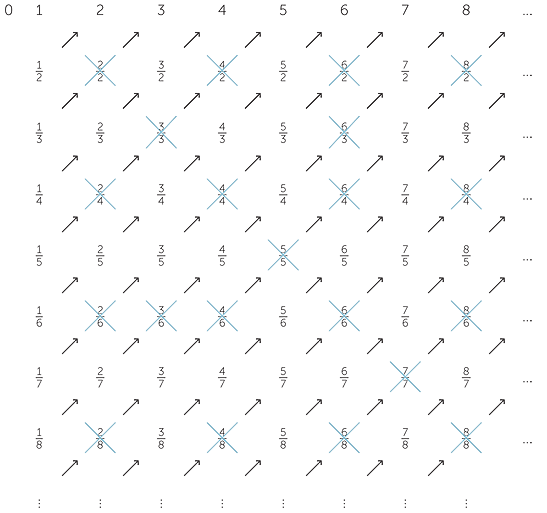
In the diagram above, every positive rational number has been written down exactly once, because the fractions that cancel have been crossed out. We can now write down all the rational numbers in a list, proceeding in the direction of the arrows, and interleaving the negative rational numbers. The list begins:

As always, the important point is that every whole number occurs exactly once in the top line, and every rational number occurs exactly once in the bottom line.

We have now proven that the sets of even whole numbers, of whole numbers, of integers, and of rational numbers are all equivalent, even though each is embedded as a proper subset of the succeeding set. Once these pieces of set-theory trickery have been done, the definition of ‘equivalent sets’ may seem to be vacuous, because it now looks as if there could always be some similar trick to demonstrate that any two infinite sets are equivalent.

Thus the next result and its proof is usually a complete surprise.

Theorem

The set of real numbers is not equivalent to the set of whole numbers.

Proof

We prove this result by contradiction. Suppose, then, that the set of real numbers is equivalent to the set of whole numbers. Then there would be a one-to-one correspondence between the set of whole numbers and the set of real numbers, and we could arrange all the real numbers in a list. If we represent each real number by its decimal expansion (excluding repeating 9s), the list would look something like this:

0 3.641559072 ...

1 167.115902726 ...

2 28.256115294 ...

3 0.008711369 ...

4 1.125266991 ...

5 900.050411818 ...

6 55.000001251 ...

7 478.515242229 ...

8 23.152556863 ...

9 529.257188231 ...

We shall now produce a contradiction by finding a real number α that is not on the list on the right. Define α by defining the nth digit an in its decimal expansion as follows:

‘If the nth digit of the real number paired with n is 1, let an = 2. Otherwise let an = 1.’
We have underlined the nth digit of each number in the list, so given our list, the decimal expansion of α would begin α = 1.211122112….

The real number α is a well-defined real number, but it is not on the list, because it differs at its nth digit from the real number paired with n. This proves that the pairing is not a one-to-one correspondence at all, giving the required contradiction. Hence the set of real numbers is not equivalent to the set of whole numbers.

We are now justified in saying, rather more loosely, that the infinity of real numbers is vastly greater than the infinity of rational numbers. As we remarked before, one should see the real number line as a continuum, with the points joined up to make a line, whereas the rational numbers are like disconnected specks of dust scattered along it.

Algebraic and transcendental numbers

If a real number β satisfies an equation P(x) = 0 where P(x) is a polynomial with integer coefficients we say that β is an algebraic number. If a real number satisfies no such equation it is said to be a transcendental number. Clearly every rational number is algebraic. Other examples of algebraic numbers are and . The transcendental numbers include π and e.

It can be shown that as the algebraic numbers are countable. We have seen that this is not true for the real numbers. Hence there are many more transcendental numbers than algebraic numbers. See the book Numbers: Rational and Irrational, given in the references for more information on this.

REFERENCES

What is Mathematics, Richard Courant and Herbert Robbins, Oxford University Press, (1941)

Numbers: Rational and Irrational, Ivan Niven, New Mathematical Library, The Mathematical Association of America, (1961)

Continued fractions: C D Olds, New Mathematical Library, The Mathematical Association of America, (1963)

ANSWERS TO EXERCISES

EXERCISE 1

0.32258064516120.

EXERCISE 2

a =

b Between any two rational numbers there is a rational number

EXERCISE 4

a

x = a + (b − a)
xis rational
Then = is rational which is a contradiction
Therefore x is irrational

b

x − a = (b − a) since b > a.
Therefore, x > a.

− x = b − (a + (b − a))
= (b − a) > 0
Therefore a < x < b.

EXERCISE 5

a1 = 1, a2 = 2, a3 = 1.25, a4 = 1.73214285…, a5 = 1.73205081…

a =

Solving for a

2a = a +

2a2 = a2 + 3

a2 = 3

a =

EXERCISE 7

3.15

EXERCISE 8

t1 = 1, t12 = 1

t2 = , t12 = 1.25

t3 = , t12 = 1.96

t4 = , t42 = 2.00694…

t5 = , t52 = 1.9988…

EXERCISE 9

[1;1,2,1,2,…]

x = 1+

   = 1 +

x2 = 3

x =

EXERCISE 10

π = [3; 7, 15, 1, 292, 1…

First five terms

3, , , ,

EXERCISE 11

[(a, b) + (c, d)] + (e, f)	= (ad + bc, bd) + (e, f)
	= (fad + fbc + ebd, bdf)
	= (b(fc + ed) + adf, bdf)
	= (a, b) + (cf + de, df)
	= (a, b) + [(c, d) + (e, f)]

The associative law for addition holds.

EXERCISE 12

a

(1,3), ; (−56, 9), −

b

(55, 18), ; (−28, 18), −

c

(42, 44), ; (10, 44),

EXERCISE 13

(a, b)(c, d) = (ac, bd) = (ca, db) = (c, d)(a, b)

EXERCISE 14

[(a, b)(c, d)](e, f)	= (ac, bd)(e, f)
	= ((ac)e, (bd)f)
	= (a(ce), b(df))
	= (a, b)(ce, df)
	= (a, b)[(c, d)(e, f)]

EXAMPLE 15

(a, b)[(c, d) + (e, f)]	= (a, b)(cf + de, df)
	= (acf + ade, bdf)
	= (acbf + bdae, b2fd)		(using equivalence)
	= (ac, bd) + (ae, bf)
	= (a, b)(c),d) + (a,b)(e, f)

EXAMPLE 16

(a1, b1) is equivalent to (a2, b2)

Hence a1 b2 = a2 b1

(c1, d1) is equivalent to (c2, b2)

Hence c1d2 = c2 d1

For addition

(a1, b1) + (c1, d1)	= (a1d1 + b1c1, b1d1)
	= (a1d1c2b2 + b1c1 c2b2, b1d1b2d2)
	=(a2b1d1d2 +b2b1d1c2, b1d1b2d2)
	=( a2d2 + b2c2, b2d2)
	= (a2, b2) + (c2, d2)

Addition is well defined.

For multiplication

(a1, b1) (c1, d1) = (a1c1, b1d1)

(a2, b2) (c2, d2) = (a2c2, b2d2)

Also, a1c1 b2d2 = b1a2d1c1

Multiplication is well defined.

EXAMPLE 17

{…(3, 5), (6,10), (9, 15), (12, 20)…}

EXAMPLE 18

[(a, b)] + [(−a. b)] = [(ab − ab, b2)] = [(0, 1)]

Therefore the additive inverse of [(a, b)] is [(−a. b)]

Uniqueness can be shown.

EXAMPLE 19

< if and only if ad < bc

EXAMPLE 20

If (a1, b1) < (c1, d1) if and only if a1d1 < b1c1

(a1, b1) is equivalent to (a2, b2)

Hence a1 b2 = a2 b1

(c1, d1) is equivalent to (c2, b2)

Hence c1 d2 = c2 d1

a1 d1 < b1 c1

a1 d1 d2 < b1 c1 d2

a1 d1 d2 < b1 c2 d1

a1 d2 < b1 c2

a2 d2 b1 < b1 c2 b2

a2 d2 < c2 b2

 

The Improving Mathematics Education in Schools (TIMES) Project 2009-2011 was funded by the Australian Government Department of Education, Employment and Workplace Relations.

The views expressed here are those of the author and do not necessarily represent the views of the Australian Government Department of Education, Employment and Workplace Relations.

© The University of Melbourne on behalf of the International Centre of Excellence for Education in Mathematics (ICE-EM), the education division of the Australian Mathematical Sciences Institute (AMSI), 2010 (except where otherwise indicated). This work is licensed under the Creative Commons Attribution-NonCommercial-NoDerivs 3.0 Unported License.
https://creativecommons.org/licenses/by-nc-nd/3.0/